Pushing it to the edge: Extending generalised regression as a spatial microsimulation method
- University of Canberra, Australia
Abstract
This paper extends a spatial microsimulation model to test how the model behaves after adding different constraints, and how results using univariate constraint tables rather than multivariate constraint tables compare.
This paper also tests how well non-Capital city households from a survey can estimate areas within capital cities. Using all households available in Australian survey means that the spatial microsimulation method has more households to choose from to represent the constraints in the area being estimated. In theory, this should improve the fit of the model. However, a household from another area may not be representative of households in the area being estimated.
We found that, in the case that the estimated statistics is already closely related to the benchmarks used, adding a number of benchmarks had little effect on the number of areas where estimates couldn’t be made, and had little effect on the accuracy of our estimates in areas where estimates could be made. However, the advantage of using more benchmarks was that the weights can be used to estimate a wider variety of outcome variables.
We also found that more complex bi-variate benchmarks gave better results compared to simpler univariate benchmarks; and that using a specific sub-sample of observations from a survey gave better results in smaller capital cities in Australia (Adelaide and Perth).
1. Introduction
In recent years, there has been increasing recognition of the importance of regional science in fields such as economics and human geography. This has meant an increased need for small area statistics. The need for small area statistics often cannot be addressed using direct estimates from survey data because most surveys use samples that are designed to provide reliable information for national level estimates, but nothing smaller. As a result it is usually impossible to derive estimates for small areas using sample surveys, and to derive a sample that would allow estimates for small areas would be inefficient (Heady, et al., 2003).
This unmet demand for small area statistics has led to an increasing number of methods to model estimates for small areas. These methods are summarised in a number of papers (ABS, 2006; Ghosh & Rao, 1994; Pfeffermann, 2002), and include simple ratio estimation, right through to random effects and Bayesian models.
Another technique that has emerged for small area estimation is spatial microsimulation. Microsimulation uses person, family or household level microdata to model real life individual conditions. Spatial microsimulation uses the microdata to estimate the condition of persons, families or households in a specific small area. Gonzales argued that the direct estimator from a survey can be a reliable estimator for a smaller area under the assumption that the small area has similar characteristics to the larger area for which the direct estimate is reliable (Gonzales, 1973).
Spatial microsimulation goes further in ensuring that the microdata used will represent the right characteristics of the small area by applying constraints or benchmarks, which are the characteristics of that small area, in the estimation process. This is done by populating a specific small area using persons, families or households from survey data based on small area benchmarks from census data that provide an accurate picture of the population in that small area.
There are a number of techniques that can be used for spatial microsimulation, but all use the basic idea of using survey data to populate the small area subject to constraints from a Census. The most common technique for spatial microsimulation is a reweighting technique, and there are a number of reweighting techniques available (Anderson, 2007; Ballas, et al., 2005; Hynes, et al., 2007; Tanton, 2007; van Leeuwen, et al., 2009; Voas & Williamson, 2000).
While there are a number of publications describing the process of spatial microsimulation, there is nothing testing the limitations of the models. For instance, the number of constraint tables used for the spatial microsimulation is an important consideration, as too many constraints may mean estimates cannot be produced due to the complexity of the constraints; and too few constraints may mean the estimates are not reliable. This paper attempts to test a spatial microsimulation model to find out how many benchmarks can be included, and when the model starts to fail as the number of benchmarks is increased.
This paper also tests how well a spatial microsimulation model using univariate benchmarks compares to a model with multivariate benchmarks. Using multivariate benchmarks allows a model to be constrained on marginal totals (so the total number of people with a certain income and rent), which should give better estimates in the final estimation process.
The third aspect of spatial microsimulation that this paper tests is whether survey sample observations which are very different to the small area bias the estimation for the small area. This is really testing whether someone from Sydney can be used to estimate an area outside Sydney (for instance, remote Western Australia).
The model being tested, SpatialMSM, is a spatial microsimulation model that has been developed to fulfil the need for reliable small area data for research and informing Government service provision in Australia. Besides estimating small area data, this model has also been linked to another microsimulation model to estimate the effect of changes in Government policy on small areas in Australia.
The SpatialMSM model employs a generalised regression reweighting program from the Australian Bureau of Statistics’ (ABS) called GREGWT. The GREGWT algorithm uses a generalised regression technique to create initial weights and iterates the estimation until the Microdata produce an overall characteristic that closely resembles the constraints for the small area. It is used by the ABS to reweight their surveys to Australia wide and capital city benchmarks.
Broadly, on any sample survey, each respondent will be given a weight, which is the number of people in the total population that the survey respondent represents. This weight takes into account a number of adjustments made by the designer of the survey, including the sample design (any over or under sampling), any clustering used, and other adjustments to the sample.
The generalised regression reweighting method takes this initial weight, and adjusts it so that the survey unit represents people in the small area, rather than the total population. The method is described in more detail in Rahman’s paper, also included in this special edition of the journal. While Rahman’s paper outlines the technical detail of the method, what is shown in this paper is the limits of the method. So the two papers fit extremely well together.
In this paper, Section 2 outlines the data and methods in detail, Section 3 provides results and analysis, and Section 4 provides conclusions.
2. Data and methods
2.1 Data
This section describes the data that the model uses. The survey data used comes from two surveys – the 2002/03 and 2003/04 ABS Surveys of Income and Housing (SIH) Confidentialised Unit Record Files (CURFs). These two survey files are combined to maximise the sample size available for the modelling.
The second source of data is the Australian Census of Population and Housing. The Australian Census is conducted every five years, and covers every resident in Australia. It therefore provides reliable estimates of socio-demographic variables for small areas. The latest Australian Census is for 2006. The Census data is used for the benchmark tables.
There are 11 Census benchmark tables used in this version of the spatial microsimulation model (SpatialMSM/08C), and these are shown in Table 1 below. The Census benchmark tables are derived from either standard output tables from the Census available through the ABS (Basic Community Profiles and Expanded Community Profiles) or special data requests from the ABS which were developed where the information was not available from ready made ABS tables.
Benchmarks used in the procedures.
| Number | Benchmark |
|---|---|
| 1 | Age by sex by labour force status |
| 2 | Total number of households by dwelling type (Occupied private dwelling/Non private dwelling) |
| 3 | Tenure by weekly household rent |
| 4 | Tenure by household type |
| 5 | Dwelling structure by household family composition |
| 6 | Number of adults usually resident in household |
| 7 | Number of children usually resident in household |
| 8 | Monthly household mortgage by weekly household income |
| 9 | Persons in non-private dwelling |
| 10 | Tenure type by weekly household income |
-
Source: ABS Census of Population and Housing, 2006
The benchmarks were selected because they were all associated with poverty and housing stress, the two output variables. If reasonable estimates are going to be derived from the spatial microsimulation model, then it is important that the constraints are related to the final output variable. In this paper, we report on poverty, so all the benchmarks are correlated with poverty. We have also included benchmarks like mortgage paid and rent paid, as this means the weights derived using these benchmarks also give reasonable estimates of housing stress.
Note that these tables are at both Household and Person level. One of the attractions of the generalised regression method as implemented in GREGWT is that the weights are integrated, which means that person weights will sum to household weights. This is described in Bell (Bell, 2000). This also means that benchmarks can be at either person or household level.
Given that the two surveys and the census were conducted at different points in time, there are some adjustments needed so that the survey data was compatible with the Census data. First, the incomes from the surveys had to be uprated to 2006 dollar values, using changes in ABS average weekly earnings. Second, the weekly household rent and mortgage had to be uprated to 2006 dollars using the housing component of the ABS Consumer Price Index (CPI).
Other adjustments to make the survey and Census compatible included removing non-classifiable households (for example, households which contain no persons over 15 or which contain visitors only) from several of the Census tables, as non-classifiable households were not on the survey dataset. We also added people in non-private dwellings to the survey dataset, as they were in the Census data, and we wanted to be able to keep them in for analysis of older people in non-private dwellings (in particular, nursing homes). The information on people in non-private dwellings came from the Census household sample file, which is a 1 per cent random sample from the Census. The household sample file used was from the 2001 Census, as the 2006 file was not available when this work was done.
The survey files also have information for each adult in the household, but not for children. Records for children are added to the ABS survey files based on information on the number of children in a family, and their ages.
The final survey file used for the spatial microsimulation is at a person level.
The Statistical Local Area (SLA) is the spatial unit used in this paper. The SLA is one type of standard spatial unit derived by the ABS and described in the Australian Standard Geographic Classification 2006 (ABS, 2007). There were two main reasons why the SLA was used as the unit of analysis in this study. First, the SLA is the smallest unit in the ASGC where there are no substantial issues with confidentiality. The ABS randomises any cells in tables where the number of people is less than 3, and as an area gets less populous, the chance of getting too many randomised cells increases. Second, SLAs cover the whole of Australia (as opposed to Local Government Areas which do not cover areas with no local government) and cover contiguous areas (unlike some postcodes) (McNamara, et al., 2008)
2.2 Methods
SpatialMSM/08c
The reweighting process in SpatialMSM uses an iterative constrained optimisation technique to calculate weights that will, when applied to the survey data, provide the best estimates of the Census Benchmarks. The technique uses a calibration estimator initially outlined by Singh and Mohl (Singh & Mohl, 1996) and described and implemented by the ABS (Bell, 2000) in a SAS macro called GREGWT. The SAS macro program is commonly used within the Australian Bureau of Statistics to benchmark survey datasets to known population targets, generally at the national or state level. In contrast, SpatialMSM uses this process to create a synthetic household microdata file for each Statistical Local Area (SLA) in Australia, containing a set of synthetic household weights which replicate, as closely as possible, the characteristics of the real households living within each small area in Australia (Chin & Harding, 2007).
Because the reweighting process is an iterative process, there will be areas where the procedure will not find a solution. If there is no solution found after a number of iterations (which can be set by the user and for SpatialMSM is set at 30), then the process has not converged. Those SLAs where the process does not converge are usually SLAs where the population is quite different to the sample population – so for instance, industrial estates or inner city areas. For many areas, however, we found that the original GREGWT criteria for non-convergence was too strict: even after iterating 30 times and not converging, the estimate of the population for each benchmark obtained from the weights was still reasonable when compared with the benchmarks. In order to maximise the number of SLAs for which we could produce valid data, SpatialMSM uses the total absolute error (TAE) from all the benchmarks as a criteria for reweighting accuracy. If the total absolute error from all the benchmarks is greater than the population in that SLA, then the SLA is dropped from any further analysis. This is called the Total Absolute Error (TAE) criteria (rather than non-convergence). The TAE has been used in a number of spatial microsimulation models (Anderson, 2007; Williamson, et al., 1998).
In SpatialMSM, the TAE criteria was implemented by summing the differences across each benchmark; and then if the total difference divided by the population in the small area was greater than one, the area was rejected. This meant that more populous areas could experience greater error. While there is no statistical basis for this value, testing has found that it is sufficiently high to keep areas where the estimates are reasonable, and low enough to exclude areas where the estimates are unreasonable.
Using SpatialMSM/08c, we have been able to produce weights for 1214 SLAs. There were 138 SLAs where the method did not appear to work, and this was shown in the failed TAE criteria. These SLAs have been dropped from further analysis. We found that most of the SLAs with failed TAE criteria were usually industrial areas, office areas or military bases with very low population size. Therefore, the proportion of persons living in these SLAs is very small (Table 2). Only 0.7% of the total Australian population in 2006 were lost due to a failed TAE criteria. Having said this, the process did not work for many areas in the Northern Territory, and 25 per cent of the Northern Territory population had to be dropped due to failed TAE. Therefore, small area estimates for the Northern Territory from SpatialMSM/08c should be treated cautiously.
Number of SLAs dropped due to failed total absolute error.
| State/Territory | SLAs with failed TAE | Total SLAs | Percent of SLAs with failed TAE | Percent of population in SLAs with failed TAE |
|---|---|---|---|---|
| NSW | 2 | 200 | 1.0 | 0.4 |
| VIC | 4 | 210 | 1.9 | 0.0 |
| QLD | 43 | 479 | 9.0 | 0.8 |
| SA | 7 | 128 | 5.5 | 0.4 |
| WA | 17 | 156 | 10.9 | 0.9 |
| TAS | 1 | 44 | 2.3 | 0.1 |
| NT | 48 | 96 | 50.0 | 25.2 |
| ACT | 16 | 109 | 14.7 | 1.0 |
| Australia | 138 | 1422 | 9.7 | 0.7 |
-
Source: SpatialMSM/08c
Measures of accuracy
To be able to see whether the change in the model gave better or worse estimates, we needed to have some measure of accuracy. What we are interested in is some measure that is external to our model, and that we know is reliable for small areas.
This subject of validation is very difficult for any researcher conducting small area estimation. The primary reason for modelling the estimates is that there are no reliable estimates from another source, so there is nothing to compare the estimates to. Some researchers have aggregated the estimates up to larger areas to compare the results, while others have used more statistical techniques to try to derive confidence intervals
There are a number of measures that have been used by other authors to validate spatial microsimulation models. These include the Overall Total Absolute Error and derivatives from this (Tanton, et al., 2007; van Leeuwen, et al., 2009); the Z-score, which is based on the difference between the relative size of the category in the synthetic and actual populations (Voas & Williamson 2000); the slope of best fit line (Ballas, et al., 2005); and the Standard Error about Identity (Ballas, et al., 2007)
Due to the nature of the benchmarking, we know that the model will estimate variables that are already benchmarked very well. These are called constrained variables. What the model needs to be able to do is estimate variables that have not been benchmarked, since the Census can provide reliable estimates of the benchmarked variables already.
The non-benchmarked (or unconstrained) variables that will be estimated reliably with these models need to be highly correlated with the benchmark variables, otherwise reasonable estimates cannot be provided. In some ways, the choice of output variable determines the choice of benchmarks. If poverty rates using equivalised disposable household income are required as the output variable, then variables like income, labour force status, housing tenure, and number of people in the household should be the benchmarks.
The unconstrained variable used for this testing was poverty rates. Because we are looking for a measure of how well our models are predicting small area poverty rates, we also need an accurate measure of poverty for small areas. We have therefore used Census data to calculate equivalised gross income for small areas in Australia. Because the Australian Census only has income available in groups, we have chosen a poverty line of $400 per week. This was the closest group to the half median poverty line that we could get using Census data.
Poverty rates using equivalised gross household income and a poverty line of $400 per week were then calculated using the same 2002/03 and 2003/04 income surveys on which the weights are based, with the incomes inflated to 2006 dollars using the change in average weekly earnings. We then applied the weights to this data to produce regional estimates of poverty. These spatially microsimulated poverty rates are therefore calculated in exactly the same way as the Census data poverty rates, and they are unconstrained (the benchmarks included income and number of adults/children resident, used for the equivalising process, in separate benchmark tables).
The next step is to calculate how far the microsimulated estimates are from the reliable estimates from the Census. In theory, if the rates are exactly the same from each dataset, then all the data points will fall on the 45 degree line. In 2007, Ballas used a “Standard Error about Identity” to estimate variability around the line of identity (a line with intercept 0 and slope 1) (Ballas, et al., 2007). While no information was given by Ballas on how this measure was calculated, we have calculated the extent of dispersion from the 45 degree line as:
where
SEI = Standard Error about Identity
yest = estimates of poverty rates from spatial microsimulation (gross income)
yABS = estimates of poverty rates from the ABS
ABS = mean estimates of poverty rates from the ABS
This Standard Error about Identity is built based on the R squared measure that has been used as the measure of overall validity of the spatial microsimulation model (Chin & Harding, 2007, Anderson, 2007, Ballas et al., 2005). The difference between the SEI and the R squared is that the R squared is a measure based on the dispersion of the data points around a line of best fit rather than the 45 degree line.
The interpretation of the SEI is similar to the interpretation of the R squared. A higher SEI is better and 100% or 1 is the highest accuracy that can be produced since it means that our estimate is exactly the same as the Census data.
2.3 Methodological changes made
Adding additional benchmarks
In this test, two Benchmark tables were added to the existing 11 and the impact of these additional tables was analysed. The usual trade off in spatial microsimulation is that when additional benchmarks are added, the procedure has greater trouble matching all the benchmarks, and fails to converge for a greater number of areas. However, with additional benchmarks, we can find that the accuracy of the final estimates increases, as there is more data being constrained to.
The aim of this exercise is to see whether it is possible to add additional benchmarks without losing too many areas due to a failed accuracy criteria, and then see how much the additional information affects the accuracy of the final estimates.
The first benchmark table that we have added is Non schooling qualification for people aged 15 years and above. Unfortunately, the classification used in the 2006 Census was different to the classification used in the Survey of Income and Housing, and the classification in the 2002/03 Survey of income and Housing is different to that used in the 2003/2004 survey. However, what we have been able to do is aggregate the classes up to as broad a group as possible, and this means they are defined in the same way for each dataset. This means we end up with only three education levels available for benchmarking, “Bachelor degree or higher, postgraduate”, “Other post school qualifications” that contains certificates and advanced diplomas and ‘No higher degree’.
The second benchmark table added was the Occupation of Employed person aged 15 and above. Similar to the new non–school education benchmark, there was a different classification used for occupation on the Census compared to the survey. In the 2006 Census, Occupation was coded to the 2006 Australian and New Zealand Standard Classification of Occupations (ANZSCO). Both the 2002/03 and 2003/04 survey of Income and Housing use the Australian Standard Classification of Occupations (ASCO) Second Edition to code occupation. There is an occupation classification mapping to allow the ANZSCO to be recoded to ASCO, and this was used to get all the occupation data into comparable classifications (ABS, 2008).
Univariate benchmarks
For all the benchmarks currently used, we specify cross tabulations (or bivariate tables), so we are constraining on a number of variables together. Another way to specify the benchmark tables would be as univariate tables, so there is only one variable in each table, rather than two or three. We would expect that because we are constraining to simpler tables, that there would be a greater level of convergence. However, we could also expect lower accuracy, measured as a lower SEI, as the bivariate benchmarks allow constraining to marginal totals (the total number of people in one category given another category). The question will be whether the greater convergence offsets the lower accuracy.
This second exercise will examine the impact of reconstructing the SpatialMSM/08c multivariate benchmark tables into several univariate tables. Of the 11 tables in SpatialMSM/08c, 7 are multivariate tables. These benchmark tables are Age by sex by labour force status (3 variables), Tenure by weekly household rent, Tenure by household type, Dwelling structure by household family composition, Monthly household mortgage by weekly household income, Tenure type by weekly household income and Weekly household rent by weekly household income (all with two variables).
There will be 10 new univariate benchmarks tables constructed from those 7 multivariate benchmark tables. As a result we know have 14 univariate benchmark tables. Table 3 gives the list of the new benchmarks tables and their sequence in reweighting process.
List of univariate benchmarks.
| Number | Benchmark table |
|---|---|
| 1 | Labour force status |
| 2 | Age |
| 3 | Sex |
| 4 | All household type |
| 5 | Tenure type |
| 6 | Weekly household rent |
| 7 | Household type |
| 8 | Dwelling structure |
| 9 | household family composition |
| 10 | Number of adults usually resident in household |
| 11 | Number of kids usually resident in household |
| 12 | Monthly household mortgage |
| 13 | Weekly household income |
| 14 | Persons in non-private dwelling |
Limiting the source of households for the microsimulation
In the first and second exercise, we have pushed the SpatialMSM model to the edge by modifying the constraints or benchmark tables used in the process. The next exercise will push the ability of this model by using a limited set of the microdata in the reweighting process. In particular, this exercise will examine the effect of using households from a specific capital city, rather than households across the whole of Australia, to estimate small area statistics in that capital city.
This exercise is important to address the question that often comes up regarding reweighting methods for spatial microsimulation, which is whether it is acceptable to use households from all around the country to represent households in a specific small area.
Theoretically there are advantages as well as disadvantages in having the entire Australian dataset available for estimation. The main advantage is that there will be more households with different characteristics to weight to a specific SLA. On the other hand, we know that non capital-city households have different characteristics to households in capital cities, so they may not be appropriate to use for estimating SLAs in capital cities.
In this exercise we will examine the result of using households from 5 specific capital cities: Sydney, Melbourne, Brisbane, Adelaide, and Perth. Using these 5 capital cities will provide us with some confidence in our results if they are consistent for each capital city. The cities and survey sample for these cities is quite different. Sydney as the most populated capital city had around 1.5 million households in 2006 while the microdata used in SpatialMSM/08c provided around 4000 households in the sample. In contrast, Adelaide is a less populated capital city and had around 450 thousand households, represented by around 2000 households in the sample.
3. Results and analysis
3.1 Adding additional benchmarks
As expected, the additional benchmarks reduced the number of SLAs that passed the TAE test. Using only the non-school qualification table as an additional benchmark, the number of SLAs that passed our TAE test was down from 1284 to 1280, so there were only four less SLAs estimated with the additional benchmark table. Using the new occupation table as an additional benchmark reduced the number of SLAs passing our TAE test to 1262, so 22 less SLAs compared to 11 using the 11 benchmarks. Introducing both the non-schooling qualification and the occupation table as the twelfth and thirteenth benchmark tables provided only 1257 SLAs to be analysed.
Although the results met our expectations in terms of reducing the number of SLAs that passed our TAE test, the impact of these additional benchmarks on the process is not as straightforward as we thought it might be. In some areas, an additional benchmark meant that an area that failed the TAE test using 11 benchmarks was now accepted, so the new benchmark improved the estimation of that SLA. Conversely, some areas that were accepted with 11 benchmarks failed in meeting our TAE criteria once we added another benchmark.
Most of the SLAs that were affected by the additional benchmark were either in rural areas with a population less than one thousand people or inner city areas. Adding education as a benchmark meant that 13 more SLAs failed our TAE criteria, although it also meant 9 SLAs that previously failed now passed pass our TAE criteria (giving the net change of four SLAs). From the 13 SLAs that now failed the TAE criteria, only 5 came from capital city areas. These were Anstead in Queensland, Hobart-Inner in Tasmania, Ludmilla in the Northern Territory and Acton and Harrison in the Australian Capital Territory. On the other hand, adding the benchmark meant that some SLAs now passed the TAE criteria, and these included City-Inner Brisbane and Duntroon and Pialligo in the ACT.
A similar pattern appears when occupation is used as the additional benchmark. The number of SLAs that failed our TAE test increased by 25, while the number that now pass was three, giving the net change of 22 SLAs. Only 5 of the 25 SLAs that now fail the TAE test were in capital cities. These five SLAs were Nathan in Queensland, Hobart-Inner in Tasmania, Ludmilla in the NT and Acton and Hall in the ACT. None of the three SLAs that now passed the TAE criteria were from capital cities.
In terms of the accuracy of the results when compared to Census data, there was an expectation that additional benchmarks would increase the accuracy of the estimates. When we compared the estimates to the number of people who lived in a household with equivalised gross income under $400 per week, we found that the estimates were in fact no better. The addition of the occupation benchmark does increase the SEI from 93.1 per cent to 94.1 per cent, but the addition of the non-school qualification benchmark reduces the SEI to 92.6 per cent. Using both tables as additional benchmarks resulted in an SEI of 93.9 per cent (Table 4).
Summary of the impact of additional benchmarks.
| Model | SLAs with TAE < 1 | SLAs with TAE >= 1 | Measure of Accuracy |
|---|---|---|---|
| SPATIALMSM08c (11BM) | 1284 | 138 | 0.9307 |
| 11BM + non school Qualification (NSQ) BM | 1280 | 142 | 0.9268 |
| 11BM + Occupation (OCC) BM | 1262 | 160 | 0.9411 |
| 11BM + NSQ + OCC BM | 1257 | 165 | 0.9388 |
-
Source: SpatialMSM/08c applied to SIH 2002/03 and 2003/04
This slight reduction in the SEI may be because we are validating against a variable that was estimated well when we were using 11 benchmarks, so we know that poverty was highly correlated with the current set of 11 benchmarks. If we were validating using something that was correlated with one of the new benchmark variables, like educational status, then we could expect to get much better results using a set of benchmarks which included education. Essentially what this suggests is that with the 11 benchmark model, we have the best estimates of poverty; but if we also wanted to use these weights for educational status (so to look at how many people with a higher degree were in poverty), then we would need the education benchmark.
3.2 Using univariate benchmarks
As mentioned in Section 2, we expect that using univariate instead of multivariate benchmarks will increase the number of converging SLAs since it will allow benchmarking to single variables, rather than benchmarking to marginal totals (so the total in one classification given another classification). The results from this exercise reported here confirm that expectation.
Using the 14 univariate benchmarks shown in Table 3 increased the number of SLAs that passed our TAE criteria to 1329 compare to 1284 SLAs passing the TAE criteria using 11 Benchmark tables with 7 of them being multivariate (Table 5). All 45 additional accepted SLAs failed our TAE criteria when 11 benchmarks were used, so we have an extra 45 SLAs. Only 16 of these 45 SLAs are in capital cities. The 16 SLAs in capital cities included Sydney-Inner, Brisbane City-Inner, Perth-Inner, Fremantle-Inner, Darwin City-Inner and Canberra City (Civic), so they were inner city areas, which are usually particularly difficult to estimate because of the diverse nature of the population in inner city areas.
Summary of the impact of using univariate benchmarks.
| Model | Accepted SLAs with TAE < 1 | SLAs with TAE >= 1 | SEI |
|---|---|---|---|
| SPATIALMSM/08c (11BM) | 1284 | 138 | 0.9307 |
| Univariate BM | 1329 | 93 | 0.8781 |
| Univariate BM and 1284 SLAs converged in SPATIALMSM/08c | 0.9100 |
-
Source: SpatialMSM/08c applied to SIH 2002/03 and 2003/04
Because the procedure is now only benchmarking to single variables (so we are not benchmarking to marginal totals), the SEI when compared to reliable Census poverty rates has reduced. We now have an SEI of 87.8 per cent, down from 93.1 per cent (Table 5). However, this may be due to the fact that there are more SLAs accepted under our TAE criteria. Using the SLAs that were accepted when we were using 11 Benchmarks, the SEI with the univariate benchmarks is around 91.0 per cent. So the reason why we get more SLAs passing our TAE test using univariate benchmarks may be that the weights calculated are good for deriving estimates of the constrained variables (which the TAE test uses), but not for deriving estimates of the non-constrained variables (which the SEI measures).
3.3 Limiting the source of households
The next exercise is to analyse the effect of using all households in the survey dataset to derive estimates for small areas that may be very different from the area that the survey respondent is in. For instance, in Australia, using a survey respondent from remote New South Wales to derive an estimate for Central Sydney. This is the default method for SpatialMSM (so the whole dataset is used to estimate every SLA in Australia).
This will be tested by looking at whether different results, in terms of the number of SLAs passing our accuracy criteria and the SEI, are achieved when a sub-population from the survey is used. The survey data allows us to identify where the respondent came from (capital city and State). This allows us to form a subset of the sample that consists of only people in Sydney, Melbourne, Brisbane, Adelaide and Perth. We then use this subset of the sample to estimate all SLAs in these capital cities; as well as using the whole dataset to estimate SLAs in each of these cities. The results are then compared to see which sample gives better results.
Source of households to populate SLAs in five capital cities.
Source: SpatialMSM/08c applied to SIH 2002/03 and 2003/04
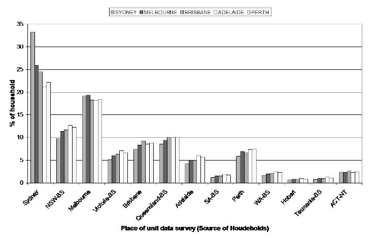
Figure 1 shows how the sample for the 2002/03 and 2003/04 Surveys of Income and Housing are distributed. What this graph shows on the horizontal axis is the location that the respondent on the survey lived in (Sydney, NSW Balance of State, Melbourne, Victoria Balance of State, etc); and then the bars show the proportion of households used from this area to provide estimates for five capital cities in Australia (Sydney, Melbourne, Brisbane, Adelaide and Perth).
What the graph shows is that to estimate areas in Sydney, about 32 per cent of respondents came from Sydney; 10 per cent came from NSW – Balance of State; 19 per cent came from Melbourne; 5 per cent came from Victoria – Balance of State; about 7 per cent came from Brisbane; 8 per cent came from Queensland – Balance of State; 5 per cent came from Adelaide or Perth; and 2 – 3 per cent came from each of South Australia – Balance of State, Western Australia – Balance of State, Hobart, Tasmania – Balance of State and ACT/NT. All these add up to 100 percent of households.
Essentially, if we were using just Tasmanian observations to estimate values for SLAs in Tasmania, we would be using far fewer households than if we use all households across Australia. So using all households gives a much more diverse set of households for the spatial microsimulation procedure to use for smaller States.
While this background information suggests that better results will be gained using all households, simply because it increases the number of households available to fill a small area, the exercise that confirms this would be to look at the SEI and the change in the number of SLAs with a TAE > 1 using all households and then using only households in the capital cities being estimated.
The results of the exercise using five capital cities in Australia are shown in Table 6. This table suggests that the results for larger cities do not depend on the sample used, but the results for the smaller cities may. There is very little difference in the number of SLAs with a TAE less than one, and the Measure of Accuracy is only different for Perth and Adelaide.
Effect of using households from each capital city to estimate areas in the capital city using spatial microsimulation.
| Source of data for estimation with SPATIALMSM/08c (11BM) | Number of sample used | Accepted SLAs with TAE < 1 | SLAs with TAE >= 1 | SEI |
|---|---|---|---|---|
| − Sydney for Sydney | 2831 | 63 | 1 | 0.9676 |
| − Australia for Sydney | 23,031 | 63 | 1 | 0.9618 |
| − Melbourne for Melbourne | 3129 | 78 | 1 | 0.9263 |
| − Australia for Melbourne | 23,551 | 79 | 0 | 0.9511 |
| − Brisbane for Brisbane | 1778 | 214 | 1 | 0.9263 |
| − Australia for Brisbane | 23,668 | 212 | 3 | 0.9224 |
| − Adelaide for Adelaide | 1824 | 55 | 0 | 0.9735 |
| − Australia for Adelaide | 23,603 | 55 | 0 | 0.9534 |
| − Perth for Perth | 1999 | 35 | 2 | 0.8478 |
| − Australia for Perth | 23,552 | 35 | 2 | 0.7856 |
-
Source: SpatialMSM/08c applied to SIH 2002/03 and 2003/04
For four out of five capital cities, using households from their own city has increased the SEI marginally with little effect on the number of SLAs passing the TAE criteria. Melbourne is the only capital city where the results show a decrease in the SEI when households from Melbourne are used to estimate Melbourne SLAs. Perth has the highest increase in the SEI with a six percentage point increase. This is followed by Adelaide where the SEI increased by two percentage points. The fact that the SEI has increased more in the two most unpopulated capital cities used in this analysis may be because the Australian sample for the two smaller capital cities used is dominated by households from the larger capital cities (see Figure 1).
4. Conclusions
This paper has made a number of changes to a spatial microsimulation model to test the effect on the number of areas that can be used from the model, and the accuracy of the estimates compared to reliable Census data. The aim is to test the reliability and stability of the model. What we have found is that the spatial microsimulation model using GREGWT is very stable. We tend to get very similar results in terms of the SEI (our measure of accuracy against the Census data) when we add benchmarks or limit the sample being used in the estimation. We have also found that using univariate benchmarks gives us more SLAs which pass our TAE < 1 criteria, but at a significant cost in terms of the accuracy of the model.
The two benchmarks that we have added in this paper did not have a huge effect on the number of SLAs with a TAE < 1, but did decrease the SEI when using poverty rates. This may be different if we were using an output variable that was correlated with the new benchmark being added.
The advantage of adding benchmarks is that the weights become more general, so they can be used to estimate a wider range of variables. The model with education as a benchmark can be used to estimate poverty rates, housing stress, and Austudy (Australian educational assistance) recipients; whereas the model without the education benchmark would only provide reasonable estimates of poverty and housing stress, as there is no education benchmark.
We found that simplifying the benchmarks by creating a number of univariate tables gave many more useable SLAs (as shown by more SLAs with a TAE < 1), but the SEI reduced. So there were advantages in benchmarking to more complicated bivariate tables.
In terms of the theory that using all households in a survey will give worse estimates for small areas, we find that the effect of using all households in Australia on the number of SLAs with a TAE < 1 and the SEI is very small. Using observations for the whole of Australia has a greater detrimental effect on the SEI for Adelaide and Perth, possibly because many of the observations in the survey come from the larger capital cities.
The implications of these results for the SpatialMSM spatial microsimulation models are:
The choice of benchmarks in a model is important. Adding new benchmarks will affect the number of SLAs that can be used; but should also mean that the weights calculated are more general.
Multivariate benchmarks are better than univariate benchmarks. The number of usable SLAs will be higher with univariate benchmarks, but estimates of partially constrained variables will be much worse.
Using all observations from the dataset will have little effect on areas where the survey has a reasonable sample size, but if estimates are being derived for areas with a small sample size, using only observations from that area for the spatial microsimulation model should give better results.
Looking at future work, these tests have all been done using one spatial microsimulation model, SpatialMSM. It would be useful to test other methods to see whether they give similar results, or whether the results are only applicable to the SpatialMSM model.
References
-
1
http://www.nss.gov.au/nss/home.NSF/533222ebfd5ac03aca25711000044c9e/3a60738d0abdf98cca2571ab00242664/$FILE/May%2006.pdfA guide to small area estimation -Version 1.0.
- 2
-
3
Census of Population and Housing: Link Between Australian Standard Classification of Occupations (ASCO) Second Edition and Australian and New Zealand Standard Classification of Occupations (ANZSCO)1232.0.
-
4
Creating small-area Income Estimates: spatial microsimulation modellingLondon: Department for Communities and Local Government.
-
5
Creating small area income deprivation estimates for Wales: Spatial microsimulation modellingColchester: University of Essex.
-
6
SimBritain: a spatial microsimulation approach to population dynamicsPopulation, Space and Place 11:13–34.
-
7
Using SimBritain to Model the Geographical Impact of National Government PoliciesGeographical Analysis 39:44–77.
-
8
Building a dynamic spatial microsimulation model for IrelandPopulation, Space and Place 11:157–172.
-
9
GREGWT and TABLE macros - Users guide. UnpublishedGREGWT and TABLE macros - Users guide. Unpublished.
- 10
-
11
SpatialMSM -NATSEM’s small area household model for AustraliaIn: A Gupta, A Harding, editors. Modelling our future: Population ageing health and aged care. Oxford: Elsevier. pp. 563–566.
- 12
-
13
Proceedings of the Social Statistics Section33–36, Use and Evaluation of synthetic Estimates, Proceedings of the Social Statistics Section, American Statistical Association, USA.
-
14
Model-Based Small Area Estimation Series No. 2 - Small Area Estimation Project ReportLondon: Office of National Statistics.
-
15
A spatial microsimulation analysis of methane emmissions from Irish agricultureRural Economy Research Centre.
-
16
Child social exclusion: an updated index from the 2006 Censuspresented at, 10th Australian Institute of Family Studies Conference, Melbourne, 9–11 July.
-
17
Small area estimation -new developments and directionsInternational Statistical Review 70:125–143.
-
18
Understanding calibration estimators in survey samplingSurvey Methodology 22:107–115.
-
19
The Australian Spatial Microsimulation Modelpresented at, First General Conference of the International Microsimulation Association, Vienna, 20–22 August 2007.
-
20
Comparing two methods of reweighting a survey file to small area data: generalised regression and combinatorial optimisationpresented at, 1st General Conference of the International Microsimulation Association, Vienna, Austria.
-
21
Microsimulation as a tool in spatial decision making: simulation of retail developments in a Dutch townIn: A Zaidi, A Harding, P Williamson, editors. New frontiers in microsimulation modelling. Vienna: Ashgate. pp. 97–122.
-
22
An evaluation of the combinatorial optimisation approach to the creation of synthetic microdataInternational Journal of Population Geography 6:349–366.
-
23
The estimation of population microdata by using data from small area statistics and samples of anonymised recordsEnvironment and Planning A 30:785–816.
Article and author information
Author details
Acknowledgements
This paper has been funded by a Linkage Grant from the Australian Research Council (LP775396), with our research partners on this grant being the NSW Department of Community Services; the Australian Bureau of Statistics; the ACT Chief Minister’s Department; the Queensland Department of Premier and Cabinet; Queensland Treasury; and the Victorian Departments of Education and Early Childhood and Planning and Community Development. We would like to gratefully acknowledge the support provided by these agencies.
Publication history
- Version of Record published: December 31, 2010 (version 1)
Copyright
© 2010, Tanton and Vidyattama
This article is distributed under the terms of the Creative Commons Attribution License, which permits unrestricted use and redistribution provided that the original author and source are credited.