Validating a dynamic population microsimulation model: Recent experience in Australia
- University of Canberra, Australia
Abstract
Available published research on microsimulation tends to focus on the results of policy simulations rather than upon validation of the models and their outputs. Dynamic population microsimulation models, which age an entire population through time for some decades, create particular validation challenges. This article outlines some of the issues that arise when attempting to validate dynamic population models, including changing behaviour, the need to align results with other aggregate ‘official’ projections, data quality and useability. Drawing on recent experience with the construction of the new Australian Population and Policy Simulation Model (APPSIM), the article discusses the techniques being used to validate this new dynamic population microsimulation model.
1. Introduction
Across much of the industrialised world, microsimulation models have become indispensable tools to policy makers. The modern welfare state today typically consists of a plethora of overlapping tax and outlay programs designed to meet multiple social policy objectives -including income redistribution and ensuring that most citizens enjoy an adequate standard of living and have reasonable access to such social services as health and education. These objectives are met through a very wide range of policy instruments, including both means-tested and universal cash transfers or service provision; means-tested and/or categorical eligibility for various tax concessions; and publicly-mandated insurance schemes or payments to be made by employers, employees or individuals. In an environment of such complexity, it is not surprising that policy makers attempt to reduce some of the risk associated with unintended or unexpected outcomes from policy change by using microsimulation models.
Microsimulation is a technique used to model complex real life events by simulating the actions and/or impact of policy change on the individual units (micro units) that make up the system where the events occur. Microsimulation is a valuable policy tool used by decision makers to analyse the detailed distributional and aggregate effects of both existing and proposed social and economic policies at a micro level.
Static arithmetic microsimulation models that simulate the immediate or ‘morning after’ distributional impact upon households of possible changes in tax and transfer policy are today the most widely used type of microsimulation models. However, in recent years many of the key policy challenges faced by the welfare state have required a much longer term perspective than that typically embodied in static microsimulation models (Cotis, 2003). In particular, the phenomenon of structural population ageing where, in decades to come, a relatively smaller proportion of taxpayers will have to support a relatively larger proportion of retirees, has created a desire among policy makers to look at policy consequences five or more decades into the future. In essence, in many countries there are grave doubts about the extent to which generous cash transfer programmes for retirees or highly subsidised health and aged care services will continue to be affordable (for recent examples from across the world see Harding and Gupta, 2007a; Gupta and Harding 2007; and Zaidi et al, 2009).
In this environment, dynamic population microsimulation models have slowly become more popular, driven not only by concerns about population ageing but also due to improvements in computing power and in data availability. Dynamic microsimulation models were the brainchild of Guy Orcutt who, frustrated by the macroeconomic models of the day, proposed a new type of model consisting of interacting, decision-making entities such as individuals, families and firms (1957, 2007). Dynamic models move individuals forward through time, by updating each attribute for every individual for each time interval. Thus, the individuals within the original microdata or base file are progressively moved forward through time by making major life events – such as death, marriage, divorce, fertility, education, labour force participation etc. – happen to each individual, in accordance with the probabilities of such events happening to real people within a particular country. Thus, within a dynamic microsimulation model, the characteristics of each individual are recalculated for each time period.
Particularly within the past 10 to 15 years, dynamic population microsimulation models have flourished, with these complex models typically moving a large sample of an entire population forward through time, for perhaps 50 to 100 years. Such dynamic microsimulation models have played a central role in government policy formation in many countries, including DYNACAN (used for Canada Pension Plan projections (Morrison, 2007, 2009)); DYNASIM, CBOLT and MINT in the US (used to inform the decisions of Congress and policy players about future welfare and tax policies (Butrica & Iams, 2000; Favreault and Sammartino, 2002; Sabelhaus and Topoleski, 2006)), MOSART in Norway (Fredriksen & Stolen, 2007), SESIM in Sweden (Sundberg, 2007; Klevmarken & Lindgren, 2008); Destinie within France (Blanchet & Le Minez, 2009); PENSIM within the UK Department of Work and Pensions (Emmerson et al., 2004); and MIDAS in Belgium (Dekkers, 2010). Such models are being used to shed light on the likely future costs of welfare state programs and the distributional impact of possible changes. For example, in Sweden, projections suggested that their retirement pension scheme would be unaffordable in the future and the government successfully legislated to reduce future benefits and increase the age at which retirement pensions became payable (Flood, 2007). Australia itself began a five year project in late 2005 to construct a dynamic population microsimulation model, the Australian Population and Policy Simulation Model (APPSIM) (covered in more detail below).
Interestingly, despite the growing interest in dynamic and other types of microsimulation models, literature on validating the results of microsimulation models is relatively sparse. To give one example, international conferences of the microsimulation community in 1993, 1997, 1998, 2003 and 2007 have resulted in six edited volumes, which together provide a very good overview of the state of microsimulation and its development over the past two decades or so (Harding, 1996; Gupta & Kapur, 2000; Mitton et al., 2000, Harding & Gupta 2007b; Gupta & Harding, 2007 and Zaidi et al, 2009). Yet, almost all of the dozens of chapters in these books focus upon the results of policy simulations, with only a handful dealing with validation issues (most notably the excellent chapter by Caldwell and Morrison, 2000). As Wolfson noted, the US National Academy of Science, in a specially commissioned panel study on microsimulation for public policy purposes in 1991, highlighted two major problems with microsimulation – validation of model results and provision of adequate data (2000, p. 155). Almost a decade after this review, Wolfson observed that the National Academy panel’s recommendations on validation seemed ‘generally not to have been followed’ in the US and elsewhere (2000, p. 162).
Even today, two decades after the US review, there is still relatively little guidance available to researchers about how best to validate microsimulation models, with one notable exception being the comprehensive description by Morrison of DYNACAN’s experience with the validation of longitudinal microsimulation models (2008). This article thus aims to share key aspects of NATSEM’s experience on the validation of dynamic population microsimulation models. This experience is based on the construction of the APPSIM model (which is still being built); the construction of the earlier DYNAMOD dynamic microsimulation model at NATSEM (King et al, 1999; Kelly & King, 2001); and almost two decades of experience with the exacting user demands placed upon NATSEM’s STINMOD static microsimulation model (Lloyd, 2007).
Section 2 of this paper describes the types of output produced by dynamic population microsimulation models and why they present such unusually difficult challenges to validate. Section 3 summarises the structure of the APPSIM model and Section 4 describes measures taken to assist in the validation of APPSIM. Section 5 provides some additional detail on the alignment measures taken in APPSIM, while Section 6 concludes.
2. Validating dynamic models
The term ‘validation’ is used here in a very broad sense, implying the need to produce a high quality product, which is one with a high level of fitness for use that is free from manufacturing defects and conforms to the design specifications (Montgomery, 1991). As Caldwell and Morrison observe: Validation is a proactive, diagnostic effort to ensure that the model’s results are reasonable and credible’ and ‘to assess whether the model’s outputs are reasonable for their intended purposes’ (2000, p. 202–203). Validation thus encompasses many distinct model development activities, embracing debugging, alignment, module specification and re-specification, quality control, checking output against sources of information external to the model, and so on.
The majority of microsimulation modellers are engaged in research with static microsimulation models, so it is worth emphasising again here why the validation of dynamic microsimulation models is a far more complex task than for static microsimulation models. A typical static microsimulation model of, say, the tax-transfer system, would first contain a cross-sectional survey snapshot of a country’s population at a particular point in time under the existing rules of the tax-transfer system and then a second ‘morning-after’ snapshot of the same population after a policy change, with these two snapshots then being compared to analyse the distributional impact of the policy change upon different types of households or individuals).1
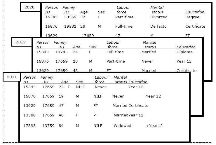
The starting point of a dynamic population microsimulation model is also typically a cross-sectional snapshot of a country’s population, although usually the sample size of this base year population is many times larger than that used in a static model (e.g. the starting year might be a one per cent sample from a population census rather than an income sample survey). The output of a typical discrete time dynamic population microsimulation model can be envisaged as also being a rectangular dataset, with a record for every individual within the model in a particular year, as shown in Figure 1.2 This figure shows a subset of three hypothetical cross-sections. The first, in 2011, shows the output for a couple family with two adult offspring. The second, in 2012, shows that the younger son has aged a year and started a part-time job, while the older daughter has grown a year older, completed a diploma, started full-time work, and married – thus creating a new family. The final snapshot shown, in 2020, indicates that that the daughter has grown older, completed a degree changed to part-time work and divorced; while the son has also grown older, completed a certificate, entered a de facto relationship and taken on full-time work.

Output structure of a typical discrete time dynamic population microsimulation model.
For a dynamic model that runs for 50 years, there will be 50 such cross-sections. This immediately creates very much larger quantities of data to store and analyse than a static model. It also creates greater validation challenges, as users will want to be able to answer the following types of temporal questions. Is income inequality likely to be greater in 50 years’ time than in 30 years’ time or than today – and, if so, why? If an age pension paid by the State is increased by a certain amount, how will this affect this inequality in 50 years time? Answering such questions exploits the capacity of the dynamic model to produce cross-sectional snapshots of the population for future years.
While the distribution of outcomes is always of interest in dynamic microsimulation, summing together the results for all individuals or large sub-groups of individuals within each year can also be a method of producing interesting aggregated time series results. For example, a policy maker might ask how much higher would be the average incomes of retirees in 2040 and earlier years if the level of a State age pension was raised.
A second way of analysing the output from a dynamic population microsimulation model is to follow individuals through time, selecting the record of a particular individual within each of the years of output (also illustrated in Figure 1). This allows longitudinal analysis of the characteristics of individuals or of the lifetime or long-term impact of policy change. This capacity can be exploited from many different perspectives. For example, it might be used to look back over the lifetimes of individuals and answer questions about the impact of divorce on asset accumulation or to determine the key defining characteristics of those with high and low lifetime incomes. Alternatively, it might be used to examine the impact of a policy change whose effects take decades to fully unfold, such as the impact on accumulated private superannuation in retirement of an increase in compulsory superannuation payments – or the effect upon lifetime earnings of an increase in participation rates in tertiary education.
The individuals can also, of course, be grouped by year or years of birth, thus allowing analysis of the changing behaviour of different cohorts – or of the impact of welfare state programs and changes in policy upon different cohorts and/or generations. Finally, the linking of the records of an individual through time allows lifecycle analysis. For example, one of the functions of the welfare state is to smooth income flows across the lifecycle of individuals, providing extra support through transfers and public services during the early lifecycle years of study and in retirement while levying higher taxes during the peak working years (Harding, 1993). A dynamic model can be used to assess how much of the redistribution generated by tax and transfer programs is simply transferring resources from one period of an individual’s lifecycle to another period, rather than transferring resources from rich to poor (Falkingham & Harding, 1996; O’Donoghue, 2002; Kelly, 2006).
Even this brief summary of the types of output typically required from a dynamic population microsimulation model illuminates the major challenges of validation that such a model creates. The model must create cross-sectional output for future years that appears credible. Often, the users will require the summed results for the individuals within the model to match external benchmarks that are considered reliable, such as official population projections. Similarly, for example, results from the Canadian DYNACAN model had to be aligned to the cell-based actuarial valuation model ACTUCAN (Morrison, 2008, p. 9). Aligning the micro values produced by dynamic models with known or projected macro aggregates usually involves some modification of model estimates. Whilst this modification does change the aggregate outputs of the model, it generally doesn’t change the distributions, preserving the microeconomic content (Anderson 2001, p. 2–6). On occasion, the aggregated results produced from other models that are trusted by policy makers conflict with one another, or are created on a different basis to the microsimulation model (e.g. by including different populations, such as those in non-private dwellings), making the task of matching the projected aggregates particularly challenging. A further difficulty is that there may be no other available projections of a variable of interest produced by a dynamic microsimulation model, so that no data exist against which to compare the model output.
While validating the cross-sectional output of future years is challenging, it is equally important that the year-to-year dynamics of individual behaviour within the model are validated to the maximum extent possible. If there are too many transitions simulated within the model – for example, too many divorces or too many periods of unemployment – then the estimates of future retirement incomes and other crucial variables will be incorrect. This is a particularly problematic area for most dynamic modellers. First, as Zaidi et al. noted when commenting on the need for further validation of the long-term trajectories of employment and earnings produced by the UK SAGE microsimulation model, ‘unfortunately there was little reliable independent data available with which to compare the simulated results’ (2009, p. 371). Second, as they also noted, period and cohort effects are also important and ‘we cannot assume that those entering the labour market in the 1990s will follow the same trajectories as the previous generation’ (2009, p. 371). This same caveat applies across many of the areas that dynamic microsimulation models seek to simulate, with the on-going long-term decline in mortality rates providing another pertinent example. Continuing changes in behaviour, in the economy, in government policy and in health status all combine to present challenges to the validation of the output of dynamic models.
The issue of changing behaviour also immediately raises the crucial importance of adequate data, as flagged by the National Academy Review in 1991 (Wolfson, 2000). Accurate estimation of the transition probabilities underlying dynamic models requires the availability of panel data, where the same individuals are tracked through time. To help in the estimation of relative rare events (such as the likelihood of having a child), a large sample is highly desirable. To assist in the evaluation of how frequently individuals change their state (such as entering or leaving the labour force or a de facto partnership), panel data that spans a significant number of years is ideally required. While there has undoubtedly been an improvement in the availability of panel data during the past decade, most researchers attempting to construct dynamic models still do not have access to all of the data that they ideally require to build and validate the model.
A final issue highlighted by the complexity of the modelling contained within a dynamic microsimulation model and of its output is the issue of useability. As Dekkers observes, a common criticism of dynamic microsimulation models is that they are a ‘black box’ (2010), and this suggests that the ease of use of the model and of assessment of its results should be a critical concern for model builders.
3. Overview of the APPSIM model
Within Australia, NATSEM commenced development of the Australian Population and Policy Simulation model (APPSIM) in 2005, with the first version due for delivery five years later in June 2010. The model is being developed with funding support from the Australian Research Council and 12 government agencies and is intended to provide an essential component of the modelling infrastructure for Australian policymakers. Credibility for APPSIM, a dynamic population microsimulation model, is critical for its continued development and acceptance within government. One essential element that is required for APPSIM to be accepted as credible is its ability to track historic data and produce projections that are reasonably consistent with other related official and non-official projections – and, where no such projections exist, the results must be plausible. This requirement ensures a significant focus on validation.
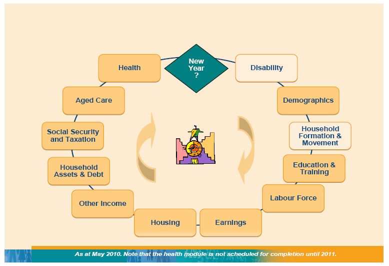
APPSIM simulates all of the major events that happen to Australians during their lifetime, on the basis of the probability of such events happening to real people in Australia. The simulated events include death, immigration and emigration, marriage, divorce, childbirth, ageing, education, labour force participation, earnings, retirement, aged care etc. Through these events, people earn income, receive social security, pay taxes and accumulate assets. The scope of the APPSIM model was unusually ambitious by international standards, with the portfolio interests of the 12 partner agencies spanning such diverse policy areas as taxation, social security, immigration, industry policy, employment, education, health, aged care, child care and child support. Not all of these interests were able to be captured within the first version of the model, but the subject areas covered are still relatively broad, as shown in Figure 2.

Outline of the processes simulated in APPSIM/2010A.
APPSIM has a similar structure to most other dynamic microsimulation models – an initial starting population, a simulation cycle and an output. (A series of working and conference papers describe the construction of APPSIM -simply go the publications section of www.natsem.canberra.edu.au and search on ‘APPSIM’.) Within the simulation cycle are sets of functions or tables of probabilities for calculating the chances of events occurring.
To calculate the probability of an event occurring, the simulation uses transition probabilities (calculated from equations or tables), based on the person’s characteristics, history and the simulated time. As the simulation clock steps through time, the chance of a person transitioning from one state to another is considered (for example changing from the state of ‘employed full-time’ to the state of ‘unemployed’). In the case of a transition between labour force states, the circumstances that influence a transition are the person’s age and sex; their labour force status in the previous two years; their educational qualifications; whether they are partnered; the age of the youngest child in the family; whether they are old enough to access their retirement savings; whether they are eligible for a government age pension; and their disability status at that time.
After calculation of a transition probability (in the range 0.0–1.0), this ‘chance’ is compared with a random number. Based on the result of this comparison, the transition may be flagged to occur. For example, if the program is run in unaligned mode, if person A’s chance of transitioning to unemployment in year t is 0.015 and a random number of 0.345 is drawn, then person A will not be flagged to transition to unemployment in year t. A feature of the model that will be discussed later is that it has the ability to adjust its outcomes to align with external reference data.
The APPSIM model is written in C#, with the simulation reading in the starting population from the 2001 Census one per cent sample file from a Microsoft Access® database. A series of Microsoft Excel® spreadsheets contain the parameters (that can be readily changed by users) and benchmarking/alignment data. Thus, in the interests of usability, every attempt is being made to ensure that key parameters are contained within the Excel spreadsheets rather than being hard-coded within the thousands of lines of C# code. A user-friendly interface allows the user to undertake such functions as selecting the start and finish years of the simulation; the percentage of the total sample to be used, and turning alignment ‘on’ or ‘off’ for individual modules.
4. Validation in APPSIM
A number of tools and features have been developed for APPSIM to ensure that the output is valid from both a cross-sectional and longitudinal perspective.
4.1 Validation mechanisms
The model has a range of tools integrated into its design to assist with the validation process. These include:
Data structure – a ‘strongly typed’ database is used and most attributes have a preset range of options;
Modular structure as shown in Figure 2;
User-selected alignment;
Individual Data Output – an output of every characteristic of a specific individual or a range of individuals and up to ten user-defined other factors at any time;
Cohort Tracking – an annual output of the characteristics of a user-defined birth cohort;
Everyone Output – every characteristic of every individual at a range of points in time (essentially cross-sectional output for future years); and
Summary Statistics – over 600 summary statistics output within each year of the simulation.
4.1.1 Data structure
The data structure that is employed within APPSIM is designed to minimise errors and quickly identify errors that do initially get through. The database that underpins APPSIM and contains all of the details on people, families and households is a ‘strongly typed’ database. This type of database uses names for each column of the database and will only accept the correct type of values. For example, internally, the column of the population database that contains a certain field is referred to as People.Columns[x] where x is the column number. However, using strongly typed fields, column 44, which contains the flag of whether a person is retired or not, uses the label RETIRED to refer to this column and the range of accepted values is limited to Boolean values of 0 or 1. This allows the programmer to refer to the retired flag as People.Retired rather than the very vague People.Columns[44]. The strongly typed field will only accept Boolean values and will reject all others.
Despite the use of strongly typed fields, previous experience with the development of dynamic microsimulation models has shown that undefined characteristics being attributed to an individual are a major source of errors. For example, the gender attribute which should have only two states (1 = male and 2 = female) can be found to be not assigned, given a value of 99 (if unknown) or, worse, it could be accidently incremented (either changing the gender from male to female or creating a new gender “3”). To minimise the possibility of assigning non-existent states to a field, APPSIM always refers to a value through an enumerator list. This ensures only valid states are used. For example, to assign a baby’s gender, the ‘sex’ enumerator list is used. This list has only two values (1 = male and 2 = female) and the coding would be baby.Gender = sex.Male or baby.Gender = sex.Female. By only referring to variable states by the enumerated value, coding mistakes and data inconsistencies are greatly reduced and almost eliminated. A final example to emphasise this point is a change in labour force status from unemployed (3) to employed full-time (1). Traditionally this would be coded as
IF person.LFST = 3 THEN person.LFST = 1.
If the value 3 (unemployed) was accidently entered as 4 (not in the labour force), it would be very difficult to identify the error. However using enumeration, the code becomes
IF person.LFST = lf.unemployed THEN person.LFST = lf.employedFullTime
and any errors in the coding (as above, if person.LFST = lf.NILF …) are minimised and easily observed and corrected.
A second major advantage of enumeration is the readability of the code. This readability makes errors easier to identify and broadens the range of people that can work on the model. Rather than coding being checked by one person and logic being checked by another, the processes can be combined and the chances of errors are reduced. In practice, this feature of APPSIM has shown itself to be of great value, with the researcher who has estimated the transition probabilities or design of a particular module being successfully able to identify errors made within the code written by APPSIM’s key programmer.
4.1.2 Modular structure
Figure 2 shows APPSIM’s modular structure – it is composed of twelve separate components which were developed separately and then coded together. The advantage of APPSIM’s modular structure is that some modules can be simulated independently of others. This allowed the developers to build modules one at a time, and to run APPSIM to check for errors as it was developed. For example, the first prototype versions of APPSIM only simulated disability demographics, household formation and dissolution, education and the labour force. The developers were then able to ensure this core set of modules worked reasonably well before moving on to subsequent modules.
4.1.3 User-selected alignment
During the initialisation of the simulation, the user has the ability to turn alignment on or off for particular modules.3 By selecting alignment ON for a given module, the outcomes of that module will align with external benchmarks set by the user. In contrast, with alignment set to OFF, the outcomes of that module will be purely an outcome of the transition probabilities or equations within that module. This allows model developers to validate the equation-generated outputs of each module in isolation. It is difficult to over-estimate the significance of alignment in a dynamic population microsimulation model that is to be used for projections by government and other agencies. For example, within the five year timeline of the existing APPSIM project, there have already been remarkable changes in both individual behaviour and government policy including, for example, sharp changes in fertility and the immigration intake. Given the time lags involved in the production of panel data and the relative rarity of some events, it is simply not possible to simulate such marked swings in behaviour or policy by re-estimating the equations underlying many of the APPSIM transitions. As a result, in many cases alignment has to be used to produce sensible results or policy change simulations. More detail is provided below on the alignment procedures used within APPSIM.
4.1.4 Individual output
The Individual Output Tool (IOT) provides an output of every field or characteristic of a specific individual along with a range of user-defined other fields at a specific point in the simulation. A group of people can be output by use of a simple loop mechanism and a person can be tracked over time by repeating the procedure each simulated year. The IOT enables each individual in scope for a transition to be output, along with the algorithm coefficients and parameters generated within the simulation at that point in time. This output provides a valuable source dataset for validation. In the case of logistic regression equation algorithms, every simulated coefficient, parameter and outcome is able to be checked and compared with theoretical or externally calculated values. Similarly, in the case of applying a distribution of outcomes based on a probability distribution, the simulated outcomes for individuals and the overall groups can be compared with theoretical outcomes for those in scope. This actual versus theoretical outcome at an individual or group level provides a very quick and thorough validation that the model is functioning within its specifications.
The IOT ability to track a person or group over time also provides a tool to observe output over time. This capability can be used to ensure that the outputs from each module and from the model overall are valid. As a dynamic microsimulation model enables the probability of an event to vary throughout a simulation, the IOT can be used to ensure that the simulated individual and group outcomes from an algorithm vary in accordance with the changing probabilities. The IOT can also be used to ensure that the correct individuals are being selected for transition. For instance, while we want a certain proportion of women to have a child in every year, we do not want the same women to be chosen each year. In other words we can use the IOT to observe the lifetime childbirths of a person and ensure these lifetime results are valid as well as the cross-sectional results.
The output provided by IOT is available with the enumerated values discussed above. This ‘plain language’ output allows simple computerised checking or a visual inspection to be undertaken to quickly identify errors in the data. For example, if the gender column is being checked, the only valid values are male and female. A value like ‘99’ will be easily detected using visual inspection of the data or the production of a frequency table.
4.1.5 Cohort tracking
The group output feature of the IOT is used in conjunction with user-input birth cohort parameters to provide a detailed cohort tracking mechanism. The ability to track a cohort enables ‘age’, ‘period’ and ‘cohort’ effects to be disentangled and validated4.
4.1.6 Everyone Output
By expanding the group feature to include everyone, the IOT output can be used to track every individual over their lifetime and validate their life path. Alternatively, by aggregating every individual within a year, the simulation outcomes sum to create a cross-sectional snapshot of the population, which can be compared with national demographic and other benchmarks.
A sample extract of ‘everyone output’ is provided in Figure 3. It shows the person ID, sex, age, place in the household, year of arrival in Australia (0 for Australian-born), student status, highest qualification, hours worked per week and marital status. At the time of writing this article, Everyone Output contains 122 units of information about each individual for each year of the simulation.
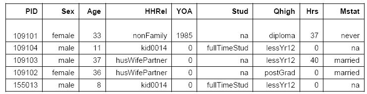
Extract from APPSIM ‘everyone output’ for Year t.
4.1.7 Summary statistics
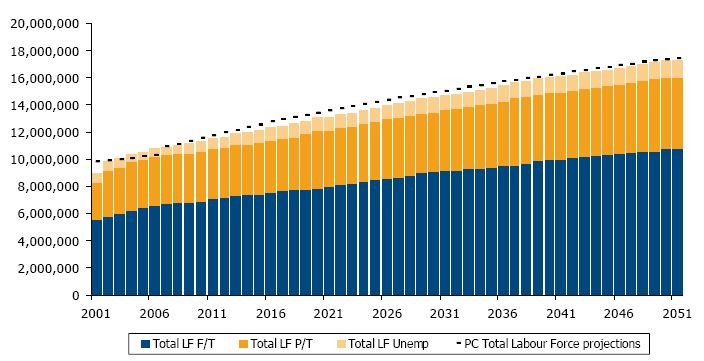
There are currently 672 summary statistics that are output each simulation cycle by APPSIM. This includes 22 population statistics (population by sex and age group), 480 labour force statistics (population by age group, sex, labour force status and highest education qualification) and 170 general statistics for the simulated year t (total population; total immigrants; average earned income; births to mothers in various age groups; women aged 30, 40, 50 with parity equal to 0, 1, 2, 3, 4, 5+; total superannuation guarantee contributions; total hospital admissions, etc). The summary statistics are output into a Microsoft Excel® workbook at the end of the simulation run. The workbook also contains external reference data and a baseline simulation output. (See Figure 4 below for a sample of one of the labour force charts output from APPSIM.) Each worksheet within the workbook combines current simulation output with the baseline simulation output and reference data in a series of charts to allow easy checking and analysis of the simulation output.

Sample labour force output from APPSIM’s automatically generated summary statistics report.
Note: the labour force output here is unaligned. The black dotted lines are labour force projections from a 2005 Productivity Commission report.
This summary statistics output is the most user-friendly output of APPSIM (similar in concept to DYNACAN’s Results Browser – Morrison, 2006). Users who do not require complex, in-depth analysis of results can simply look at the charts, rather than analyse the ‘everyone output’ themselves by using a statistical package such as SAS or STATA. Furthermore, summary statistics make validation easer, as modellers can tell quickly whether their aggregate output appears reasonable or not. There is a time cost to the production of this user friendly output, although our initial calculations suggest that this cost is only a few minutes per year of simulation, with a simulation of the full database (of some 200,000 individuals in the start year) for 50 years currently taking more than 12 hours to run5. However, one of the lessons from NATSEM’s earlier experience with the DYNAMOD dynamic microsimulation model and from on-going experience with the STINMOD static microsimulation model is that it is essential that a model be made as accessible to non-programmers as possible. While there will always be a handful of sophisticated users who require access to source code and who have the skills to analyse complicated output datasets, constant turnover of staff within client agencies means that it is essential to do everything possible to facilitate usage and training if a microsimulation model is to stay ‘alive’.
4.2 The APPSIM validation experience
APPSIM’s validation process was loosely based on that outlined by Rick Morrison in the development of DYNACAN (2008): that is, it focused on data/coefficient/parameter validation, algorithmic validation, module-specific validation, multi-module validation and impact validation. Both cross-sectional and longitudinal data were used as reference data.
Most cross-sectional data used as benchmarks for validation came from the Australian Bureau of Statistics, including the Labour Force Survey, births, migration data and so forth. Some reports from other government departments were used to benchmark long-term projections, such as Treasury’s Intergenerational Report series (the most recent being for 2010).
The only major longitudinal survey of the general population in Australia is the Household, Income and Labour Dynamics in Australia Survey6 (HILDA). The HILDA Survey is a household-based panel study which began in 2001. HILDA is funded by the Australian Government for at least 12 waves and is managed by the Melbourne Institute of Applied Economic and Social Research. While HILDA enables a range of longitudinal issues to be considered and modelled in APPSIM, it is limited by its small size (wave 1 consisted of 7,682 households and 19,914 individuals); the short life of the survey (only seven waves available in 2009); and that some topics are not surveyed every year (for example, household assets were only surveyed in 2002 and 2006). The majority of the transition probabilities and logistic regression equations in APPSIM have been derived using data drawn from this survey, and its distributional information and transitions have been used for validation.
Data/Coefficient/Parameter validation
This stage of validation included examining the initial databases to ensure that the base data for the model are reasonable. This should be the first stage of validation – even if a model is perfect, it will produce unreliable results if it is based on incorrect data.
Since APPSIM’s base data was based on a 1 percent sample of the 2001 census, there was reasonable certainty that the core of the base data was robust. Some values had to be imputed into the base data, such as the precise level of earnings and superannuation savings. Most imputed values were derived from HILDA data, and aggregate values and distributions were validated using ABS data. The strongly typed database made this stage of validation much easier than it otherwise would have been.
As with most dynamic models, extensive effort was devoted to the stages of reviewing the structure of modules within other dynamic models; designing an appropriate structure for each process included within APPSIM; estimating the equation coefficients, and devising appropriate alignment parameters (see the Working Papers on the NATSEM website for details of the construction of individual modules).
Programmers’/Algorithmic Validation
This stage of validation simply involves ensuring that the model’s code does what it is supposed to do. It proved to be a vital stage in APPSIM as, in most cases, the developer of the module was not the same person who wrote the code for it. In developing APPSIM’s modules, the module’s creator sent a description of the model and parameter spreadsheets to the coder, who then wrote the module in C#. Typically, algorithmic validation occurred in APPSIM with the module creator examining the code with the assistance of the coder, and ensuring that the model was coded in the way that they intended.
An example of this in APPSIM’s development was that very early labour force simulations showed very low levels of labour force participation. When the labour force modeller read through the code, she realised that the impact of disability on labour force participation had been coded ‘backwards’; that is, 10 represented no disability and 0 represented profound disability, when the module was designed for 0 to represent no disability and 10 profound disability. The strongly typed data structure made the code much easier for the module designer, who was not fluent in C#, to read.
Module-specific validation
This is the first type of validation that requires running the model and analysing its outputs. The optimal method for performing module-specific validation is to align all modules except for the target module, and switch alignment off for the target module. Assuming the alignment works, this will allow the developers to test the validity of each individual module. This form of validation is essential before moving towards multi-module validation, as one can be reasonably sure that errors in the model output are due to flaws in the module under examination. For example, if a modeller examines unaligned output to validate the labour force module and finds that labour force participation is too low, it could be that the labour force module is mis-specified, or it could be that errors in the education, family formation, births or disability modules are affecting labour force participation, as all these modules provide inputs into labour force participation. Holding the other modules constant allows the modeller to be sure that any unexpected results are due to the structure of the labour force module.
A dynamic microsimulation module ideally needs to be validated in at least two dimensions – cross-sectionally and longitudinally. This section discusses our experience in the validation of the labour force module as an example of the issues raised for model developers.
Cross-sectional validation
This involves comparing aggregate and distributional output from individual years in the model to external benchmarks – for example, the total population in a given year or the number of people in the labour force. These can be short-term or long-term benchmarks. The benchmarking data must have sufficient detail to determine if the distributional output of the module is reasonable, as well as the aggregate output. This form of validation in APPSIM relies heavily on the automatically-generated Excel summary outputs and the ‘everyone output’ described earlier.
The short-term validation of the labour force module – using 2006–2009 data – was performed using data from the Australian Bureau of Statistics’ Labour Force series and the HILDA survey. The Labour Force series has a much larger sample, is released more frequently and is released more quickly than HILDA, so this was used where possible. Where the Labour Force series did not go into sufficient detail, HILDA was used.
The module developer ran an APPSIM simulation with all modules except for the labour force aligned. The output from this simulation was then compared with the external benchmarking data. If APPSIM’s output differed substantially from the external data, the equations were revisited and edited, and the simulation run again until the external benchmarks were more fully met. Validation benchmarks included:
Labour force status by sex, age and full-time student status;
Retirement status by sex for all persons aged 55+;
Hours worked per week by sex and labour force status; and
Self-employment by single year of age.
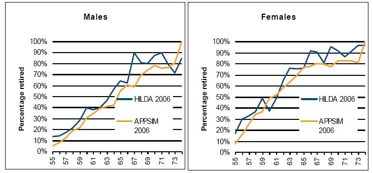
As an example of the validation outputs, Figure 5 shows the percentage of the population at each year of age from 55–74 who consider themselves retired (and in the case of HILDA, are not in work and do not go back to work after they describe themselves as retired). It compares APPSIM outputs from 2006 with 2006 HILDA data.

Percentage of people who are retired, age 55–74, APPSIM and HILDA 2006, by age and sex.
Source: APPSIM simulations, HILDA 2006.
These retirement rates simulated by APPSIM line up reasonably well with those from HILDA, although HILDA data is a little ‘noisy’ due to its sample size. For both sexes APPSIM simulates retirement rates that are lower at young ages; this is largely because in APPSIM one cannot retire until one turns 55 while, in HILDA, some people retire at age 54 or earlier. APPSIM retirement rates can be expected to be slightly lower as APPSIM does not attempt to simulate the effect of some generous early-retirement pensions, which are now being phased out in Australia. Likewise, APPSIM retirement rates are slightly higher among the oldest people shown in this graph, as APPSIM assumes 100 percent retirement by age 75. The long-term cross-sectional validation of the labour force module involved comparing APPSIM outputs to long-term projections – out to 2047 -made by the ABS and Treasury. These projections were far less detailed than the short-term data available, so long-term validation was performed on the basis of labour force participation by age and sex only.
Caution must be used when comparing a dynamic microsimulation model’s output to that of external projections. Since these projections are heavily dependent on assumptions made, it should not be assumed that model output that misses the projections is necessarily a reflection of a bad model.
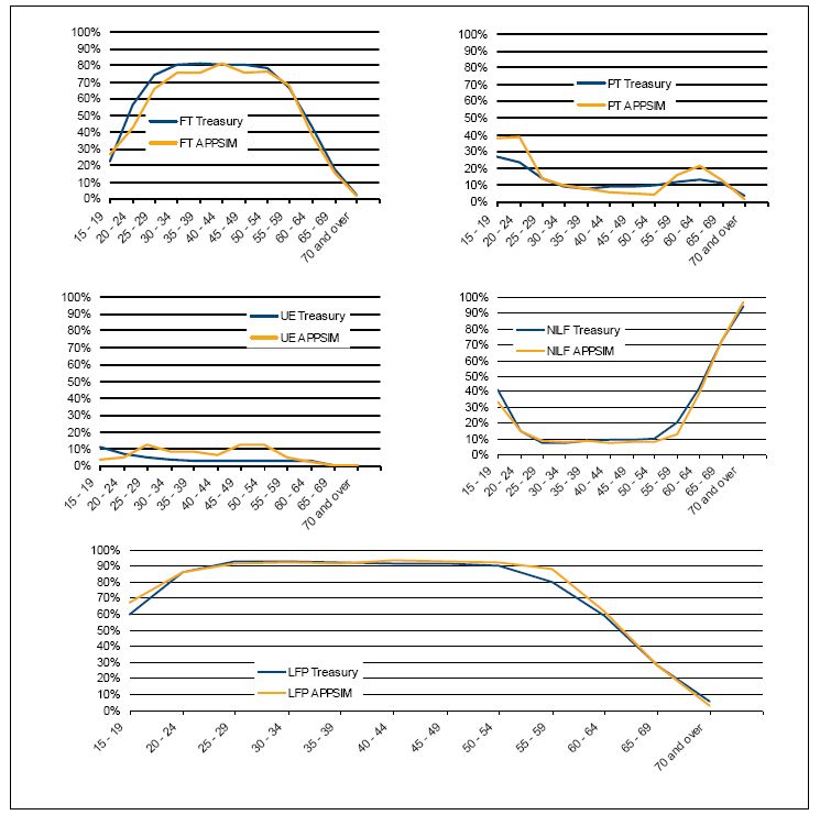
As an example, Figure 6 shows Treasury’s 2047 labour force projections of full-time and part-time workers, the unemployed, not in the labour force and total labour force participation, graphed against APPSIM’s unaligned projections of the same. For men, overall APPSIM simulations track Treasury’s simulations reasonably closely, with the exception of slightly lower full-time employment among males in their 30s and 40s, due to higher rates of part-time employment and unemployment. However, overall participation patterns are reasonably similar to Treasury projections. The main difference in labour force participation is that Treasury projections show labour force participation starting to decline among men in their fifties, while APPSIM shows men maintaining high rates of labour force participation up until their sixties. This is due to a key assumption made by the APPSIM labour force model which is that, as the age at which one can access superannuation increases to age 60, men will be much more likely to remain in the labour force until they are out of their fifties. It should be noted that Treasury has recently released revised labour force projections as part of its latest Intergenerational Report, which provides a pertinent illustration of how the external benchmark data against which the output of a dynamic microsimulation model is being evaluated can change relatively rapidly (2010).

Labour force states of men in 2047, APPSIM and treasury projections.
Source: Treasury (2007) and APPSIM simulations.
Longitudinal validation
The longitudinal validation process typically involves assessing the validity of rates of change in individual states over time, the frequency of transitions or the number of transitions in a lifetime. This validation is essential to ensure that the model is fit for purpose, but is often extremely difficult to actually do. For example, cross-sectional validation may show that the correct number of people are in the labour force each year, but the model will be useless if most of the individuals within it change their labour force status every year when, in real life, most people retain the same labour force state from one year to the next.
Longitudinal validation requires benchmarking data that either follows individuals or groups of individuals over time, or recall surveys that ask individuals about events that have happened over the course of their lives, or relies on expert opinion about the likely number of events or transitions in a lifetime (such as that provided by demographers). Recall survey information will only reliable if it is likely that almost all respondents will accurately recall the life event: women’s parity data based on recall surveys will be relatively reliable as very few mothers forget how many children they have had or when they were born (although parity may have changed so much during the intervening period that the recall data may not actually be helpful for validation). Earnings data will be far less reliable if based on recall surveys, as few people will be able to accurately recall what their salary was 20 years ago.
The cost and complexity of collecting this type of data means that it is often not available, so other, less reliable sources often are used. CORSIM and DYNACAN had access to decades’ worth of administrative data for validation (Caldwell & Morrison, 2000); unfortunately no such long-term data are available to researchers in Australia. For example, determining the distribution of lifetime labour force participation would require 50 years’ worth of administrative or survey data. However, the tracking and collecting of data for this length of time would generally be prohibitively expensive, Australian government departments have no reason to store such data for more than a decade, and the information may be tainted by cohort and period effects.
The HILDA survey has been of great use in validating some parts of APPSIM longitudinally. However, its deficiency relates to its short life to date. The small number of waves makes it difficult to separate out the age, period and cohort effects from the underlying trends and behaviour. Even so, it has been used to determine whether year-to-year transitions in a short timeframe appear reasonable.
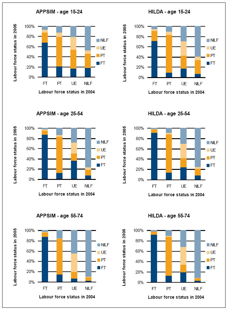
In validating the labour force module, for example, the percentages of people who transitioned between labour force states between 2004 and 2005 in HILDA and APPSIM were compared. This was accomplished by merging two years’ worth of APPSIM ‘everyone output’ and comparing it to a specially constructed comparable HILDA file. Figure 7 shows the results. The X axis indicates a person’s labour force status in 2004 and the Y axis indicates the percentage of people who were in each labour force state in 2005, given their labour force state in 2004.

Labour force transitions in HILDA and APPSIM, 2004–2005.
Source: HILDA, APPSIM calculations.
Figure 7 shows that the distribution of labour force transitions that occurs from one year to the next in each age group is quite similar in APPSIM and HILDA. For example, consider the two centre charts, those that show APPSIM and HILDA transitions in the 25–54 age group. The APPSIM chart (on the left) shows that 88 percent of 25–54 year olds who were full-time employed in APPSIM in 2004 were still employed full-time in 2005. Eight percent of these people switched to part-time employment, two percent were unemployed and two percent had left the labour force. The HILDA chart (on the right) shows that 91 percent of people who were full-time employed in 2004 were still working full-time in 2005. Of the remainder, seven percent worked part-time, one percent were unemployed and one percent left the labour force. These charts offer some reassurance about the year to year labour force transitions simulated in APPSIM – although it should also be recognised that there is considerable ‘noise’ in the HILDA estimates due to small sample size in some groups and also that the HILDA data were collected during a period of strong economic growth, so an ability to change the APPSIM alignment parameters is essential given such factors as the recent Global Financial Crisis.
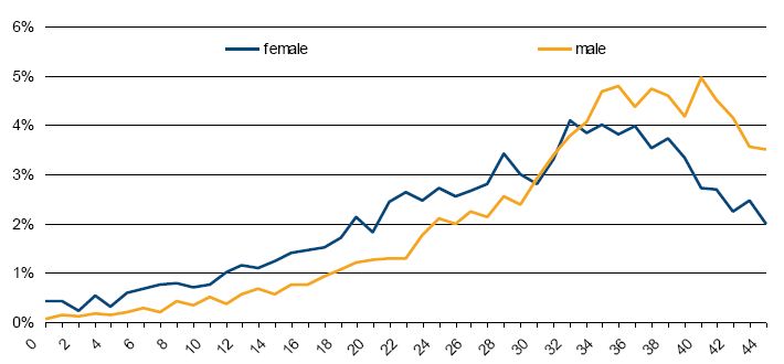
A final example of longitudinal validation is provided in Figure 8. This shows the distribution of the number of years spent in the labour force for persons born in 1981–1986 by 2051, when they are aged 65–70 years. It shows that 72 percent of males and 55 percent of females spent at least 30 years in the labour force. Although it is important to produce longitudinal output of this type, this type of APPSIM output cannot be readily compared against any other benchmark data in Australia. For example, the data in Figure 8 cannot be compared to any existing data on the total number of years that today’s 65–70 year olds spent in the labour force due to cohort effects. The best that can be done is for the model developer to assess whether the output appears reasonable.

Distribution of years spent in labour force by sex, 65–70 year olds in 2051.
Source: APPSIM simulations.
Multi-module validation
This stage of validation involves examining model outputs with results that depend on the interaction of several modules. This allows the modelers to examine the short- and long-term cross-sectional and longitudinal outputs when all the modules are able to interact. This stage of validation is necessary to ensure that reasonable results are produced when the outputs of one module are inputs into another module; and to validate outputs that are produced by more than one module; for example, the number of children living in households in which no adult has a job. Again, multi-module validation can be performed cross-sectionally and longitudinally.
Cohort tracking and the IOT have proved very useful tools in multi-module validation. Once again, ‘everyone output’ is very useful for cross-sectional validation and a few years’ worth of longitudinal validation, and IOT tables and cohort tracking are very useful for longitudinal validation. One example of this type of validation within APPSIM resulted in changes to the immigration module, after questions were raised about how the education levels of immigrants had been coded, given that the highest educational qualification input being used in the labour force module did not appear correct. Similarly, at the time of writing, extensive work is being undertaken on validating the family formation and dissolution modules, as part of the process of refining the aged care module: this is required because one of the key predictors of the need for formal aged care is the presence or otherwise of a partner who can provide informal care.
Impact validation
The first four stages of validation as discussed in this paper are dedicated towards making sure a dynamic microsimulation model is capable of producing reliable projections. The final stage, impact validation, involves ensuring that these projections can be reliably used to estimate impacts of policy changes.
If APPSIM is used to estimate the impact of a policy change, how can modellers know if this estimate is reliable? First, the modellers can ensure that the model is internally consistent. For example, if APPSIM is used to test the impact of a policy on superannuation accumulation, modellers can ensure that individual superannuation balances and household superannuation balances sum to the same amount. Second, APPSIM can be used to perform simulations that have already been performed by macroeconomic models, to see if it is able to produce the same aggregate effect. For example, if the Australian Treasury’s long-term modelling shows, hypothetically, that a two percent increase in labour force participation over the long term produces a three percent increase in total superannuation balances after 20 years, APPSIM could be tested by using alignment to simulate a similar increase in participation and comparing its increase in superannuation balances to those simulated by Treasury.
The government agencies who are NATSEM’s research partners in the APPSIM project have repeatedly stressed that they are most often interested in the difference made by a policy change (such as the change in taxation revenue) rather than the benchmark aggregate itself (such as total taxation revenue before the policy change). Their input has guided the construction of many of the summary charts produced at the end of each APPSIM simulation run.
However, our experience over more than a decade with the STINMOD static microsimulation model has shown that impact validation presents particular challenges for validation, as clients very often run a policy simulation that the NATSEM modellers have not managed to anticipate – and issues with the modelling or the data underlying the modelling often only emerge when a specific policy question is asked of the model. To this end, much of our recent research has focussed on undertaking relevant policy simulations, such as changing the Superannuation Guarantee (Keegan, 2010); examining health care costs with an ageing population (Lymer, 2009); or adjusting the age of eligibility for age pension (Harding et al, 2009).
5. Alignment in APPSIM
Alignment can be used for a number of purposes in a dynamic microsimulation model. First, it can be used in the validation process to isolate each individual module for validation. Secondly, it can be used to eliminate Monte Carlo variation between simulations. Thirdly, it allows the user to set different targets for policy simulations or sensitivity analysis; for example, determining if a policy has noticeably different impacts if a higher birth rate, wage growth rate or labour force participation rate is assumed. Finally, it can be used to ensure a module creates reasonable aggregate outputs when the unaligned outputs of the model are not considered sufficiently accurate or are out-of-date.
For example, as O’Donoghue et al. (2009) and Duncan and Weeks (2000, p. 292) have noted, the predictive ability of logit and probit models can be poor in some cases even when the model is well-specified. They attribute this to the fact that the further the probability of an event is from 0.5, the less likely the equations are to produce the desired result. In other words the simulation may under or over predict the number of events (O’Donoghue et al. 2009, p.25). Unfortunately, in the real world, few event probabilities are close to 0.5 (for example, the chance of childbirth in the next 12 months for a woman aged 15 to 49 years is 0.04) and, thus, even perfectly specified models will produce incorrect event outcomes.
Data problems are particularly pertinent to Australia. For example, some six waves of the HILDA panel data are used to estimate many of the transition probabilities within APPSIM. Given HILDA’s relatively small sample, of around 7,500 households each year, it is inevitable that the equations produced from it (particularly for relatively rare events such as childbirth) will contain some ‘noise’ (see Bacon & Pennec, 2009:20 for an example). In addition, by chance, HILDA captures a period of strong economic growth within Australia and it is not certain that the behaviour of individuals estimated from it will continue to be the same during the current economic turmoil and into the future.
Another vital reason for alignment is that projections of the future will change according to the ever-changing circumstances observed in the present. For example, the Australian Treasury released three Intergenerational Reports between 2002 and 2010 (Treasury 2002, 2007, 2010), all with different projections of future birth-rates, labour force participation and GDP growth. In the first report, the birth-rate was projected to fall to 1.6 children per woman, as it had been steadily trending downward for decades. Following the release of IGR1, the birth-rate started increasing again and reached 1.97 in 2008 (ABS 2008), so subsequent IGRs have changed their assumptions about future birth-rates. If it were not for alignment, APPSIM would have to be recoded for every change in assumption about the future. The alignment process allows users to change these assumptions quickly and easily.
5.1 Introducing variability into alignment
The international consensus about the need for alignment in dynamic population microsimulation models appears to have strengthened during the past decade or so (e.g. see Morrisson, 2008, p. 16; Kelly and King, 2001) and the debate has shifted more towards how to improve alignment techniques. In the earlier ‘simpler’ versions of alignment, every person in scope for a particular event was assigned a probability score. Then the in-scope population was ranked based on their score. In this ‘simple’ version of alignment, the appropriate number of people to make the transition were then selected, based their ranking, to match the external benchmark. This strategy effectively ensures that correct number of persons with the right characteristics experience the event. However, in the real world these events are stochastic – there is an element of randomness in who is selected to transition. As O’Donoghue et al. have noted, the model must ensure some variability, otherwise only those with high probabilities will be selected, which will not reflect reality (2009). Even a person with a low probability of becoming unemployed (for example, a married, degree-qualified, full-time employed male aged 45 years) will occasionally lose his job and become unemployed.
To replicate this randomness in the case of aligned outcomes, APPSIM uses a technique to introduce some variation into the ranking list. It does this by selecting a proportion of people and then inverting their probability scores (that is the probability score used for ranking is subtracted from one [ranking probability = 1 − calculated probability]). With an inverted probability, those that would be ranked very low are ranked very high and vice versa. The alignment ranking process is then used in the normal manner to select those who actually make the transition.
Analysis of HILDA data from 2005 to 2008 has shown the large degree of randomness that can be present in the real world. This fact was emphasised in a comparison of the probabilities of women undergoing childbirth (based on the regression equations used in APPSIM) and actually having a child (as recorded on the next wave of HILDA). As four per cent of women in this age group have a child, it could be expected that all of the actual births would have come from the highest probability quintile. In reality only 43 per cent of births came from this group and 20 per cent of births occurred to women in the lowest probability quintile. Clearly childbirth is one event that cannot rely solely on ranking probabilities for selection.
Baekgaard (2002) recommended using the difference between the probability and a random number as the ranking variable, rather than just probability, to introduce variability into the alignment selection process. However, this limits control of the degree of randomness introduced into the selection process. The method currently implemented in APPSIM provides both variability in those selected for transition and control over the amount of variation. In theory, different levels of variation could be used for different events -and a very high level of variation be used for an event like childbirth but a low level of variation be used for, say employed fathers of young children leaving the labour force. At this stage in APPSIM’s development, the level of inversion used to introduce variation is set at a single value for all events and this level of inversion is user- defined. By default, the proportion to undergo inversion is currently set at ten per cent.
5.2 Level of alignment
Another area of debate has been the level at which event alignment should occur. O’Donoghue et al. identify three levels of alignment -alignment at the level of the individual equation; ‘meso-alignment’ at the level of detailed population sub-groups; and ‘macro alignment’ at the level of larger population sub-groups (2009, p. 26). They identify a mechanism for ensuring that the various alignment totals are consistent with each other.
For APPSIM, the degree of detail used in the alignment parameters varies by module, in line with available data and key policy debates. For example, in the immigration module, macro-alignment is used to ensure that the aggregate totals match external benchmarks and then meso-alignment is undertaken by visa category proportions, as visa category is such an important policy instrument in Australia. In the labour market module, cross-sectional alignment of labour force status by sex, age and full-time student status is undertaken.
As noted in the earlier discussion in Section 4, it is important to also consider whether the outcomes of a dynamic population microsimulation model provide reasonable answers when one looks at the year-to-year dynamics and the lifetime outcomes, as well as in the cross-sectional output. Thus, this involves examining whether a reasonable number of marriages, employment transitions, education transitions and so on appear to be simulated over the longer term. Validation and any associated possible longitudinal alignment are particularly difficult in this domain, because of the typical lack of adequate data to benchmark or calibrate against. However, one area where we have experimented with improving our longitudinal outcomes is in the simulation of fertility within APPSIM. This was initially prompted by the substantial number of larger families being generated by the fertility transition equations originally estimated from the HILDA data. The alignment spreadsheet has been refined by adding parity to the fertility alignment benchmarks for each age and marital status group. Every year, once births have been initially allocated, APPSIM’s alignment process examines how many women in each age bracket have had one, two, three, four or more children. If too many women in a particular age bracket have had too many children, alignment will reallocate the births for that year so that the distribution of children among women is appropriate. Examination of the outcomes from the family formation and dissolution modules is continuing, to determine whether any special measures need to be taken to control the number of marriages, divorces, and de facto partnerships and separations.
While the above discussion has focussed on event alignment, it is also worth noting that there are other types of control totals that can be used to align to, including ‘the distribution of values and the average growth rate in the value of an event’ (O’Donoghue, 2009, p. 25). As Morrison observed, DYNACAN, for example, was required to align its earning outcomes to target distributions prescribed by the ACTUCAN model (2008, p. 16). MIDAS separates monetary alignment by sex and uses a two-stage uprating process to align earnings. This allows earnings to be aligned while still taking into account the impact of the age and sex distribution within the population on average earnings (Dekkers et al, 2010). Within APPSIM alignment to a range of monetary targets has been implemented. For example, average earnings increase at a constant rate defined by the model user. In the modelling of superannuation (retirement pension) contributions, a range of alignment techniques are used. Macro alignment is used to ensure the aggregate amount contributed matches benchmarks. Meso-alignment is used to match the proportion of people making voluntary contributions by age, sex and labour force status and the proportion of their income that each contributes.
6. Conclusions
The construction of dynamic population microsimulation models is an extremely demanding task, with the budget available for validation and documentation typically being squeezed by the sheer difficulty of the earlier tasks of determining how to model complex social processes and estimating the requisite transition probabilities associated with those processes (Harding, 2007). Drawing upon NATSEM’s earlier experience with the DYNAMOD and other NATSEM models, this paper has outlined key features of our experience with the validation of the APPSIM dynamic population microsimulation model. This focus on validation has resulted in an emphasis upon alignment mechanisms; the ability to turn alignment ‘on’ or ‘off’ for particular modules; a user-friendly interface; the placement of key alignment and transition equation parameters within easily accessible Excel spreadsheets; the automatic generation of a suite of summary output tables and charts at the end of each simulation; the creation of output datasets for ‘everyone’, specific individuals or specific cohorts; a modular structure; and a ‘strongly typed’ database to assist with code readability by those not proficient in C# and error debugging.
Footnotes
1.
While some static microsimulation models now incorporate a behavioural component (such as the change in labour supply in response to a policy shock – Kalb and Thoresen, 2009; Creedy et al, 2002) or a macro-economic response (Foertsch & Rector, 2009) the key point is that in essence generally only two or a handful of cross-sectional years of output are compared.
2.
The output of and the challenges faced by continuous time dynamic models and dynamic cohort microsimulation models are somewhat different and not discussed here, with this article only canvassing discrete time dynamic population microsimulation models.
3.
One of the referees for this article made the very interesting observation that it would be desirable to be able to turn alignment ‘on’ or ‘off’ for individual equations within each module, rather than for entire modules, as is currently the case within APPSIM.
4.
The ‘age’ effects are those where we see a distinctive pattern over the life course. For example, fertility rates are low for women under 20 years, high for those in their 20s and 30s, low again in their 40s and zero above 50 years of age. ‘Period’ effects are those that reflect the conditions prevailing at different times. For example, the returns on investments and taxation rates vary over time. ‘Cohort’ effects refer to the way in which birth cohorts of the population behave differently. For example, people who lived through the depression and were in their fifties in the 1970s may well have behaved differently to how younger cohorts will behave once they reach their fifties in the 2020s.
5.
It should be noted that no attempt has yet been made to increase the efficiency of the code. In addition, our testing to date suggests that running a simulation against a 10 per cent sample of the database produces reasonable estimates within a couple of hours, allowing the policy analyst to get an early indication of whether outputs appear sensible and an over night run of the model is justified.
6.
However, there have been a few smaller surveys that collect historical information from respondents. As the historical approach relies on the respondent accurately recalling when an event occurred, it is not generally as accurate as annually surveying participants.
References
-
1
Births Australia 2008, Australian Bureau of StatisticsBirths Australia 2008, Australian Bureau of Statistics, Cat. No. 3301.0, Canberra.
-
2
http://www.soa.org.ccmModels for Retirement Policy Analysis, Report to the Society of Actuaries.
-
3
Microsimulation, Macrosimulation: Model Validation, Linkage and Alignmentpaper presented at the, 2nd General Conference of the International Microsimulation Association, Ottawa, 8–11 June, www.microsimulation.org.
-
4
Micro-Macro Linkage and the Alignment of Transition Processes: Some Issues, Techniques and ExamplesOnline Technical paper TP25, National Centre for Social and Economic Modelling, Canberra, www.natsem.canberra.edu.au.
-
5
287–306, Projecting Pensions and Age at Retirement in France: Some Lessons from the Denstinie I Model287–306, Projecting Pensions and Age at Retirement in France: Some Lessons from the Denstinie I Model.
-
6
Divorced Women at Retirement: Projections of Economic Well-Being in the Near FutureSocial Security Bulletin, 63, 3, Social Security Administration, Office of Policy, Office of Research Evaluation and Statistics.
-
7
Validation of longitudinal dynamic microsimulation models: experience with CORSIM and DYNACANIn: L Mitton, H Sutherland, MJ Weeks, editors. Microsimulation modelling for policy analysis: challenges and innovations. Cambridge University Press. pp. 200–225.
-
8
Population ageing: facing the challenge1, Population ageing: facing the challenge, OECD Observer, No 239, September.
-
9
Microsimulation Modelling of Taxation and the Labour MarketCheltenham: Edward Elgar.
-
10
On the impact of indexation and demographic ageing on inequality among pensioners: validating MIDAS Belgium using a stylized modelPresented at the, European Workshop on Dynamic Microsimulation, Brussels, Federal Planning Bureau, March 2–5.
-
11
The long term adequacy of the Belgian public pension system: An analysis based on the MIDAS model. Working Paper 10-10Brussels: Federal Planning Bureau.
-
12
Simulating transitions using discrete choice modelsProceedings of the American Statistical Association 106:151–156.
-
13
An Assessment of Pensim2. Institute of Fiscal Studies Working Paper WP04/21An Assessment of Pensim2. Institute of Fiscal Studies Working Paper WP04/21, http://www.ifs.org.uk/wps/wp0421.pdf.
-
14
Poverty alleviation vs social insurance systems: a comparison of lifetime redistributionIn: A Harding, editors. Microsimulation and Public Policy. North-Holland: Amsterdam. pp. 233–265.
-
15
Impact of Social Security Reform on Low-Income and Older Women. AARP Public Policy Institute Report No. 2002–11Washington, DC: AARP.
-
16
33–54, Can We Afford the Future? An Evaluation of the New Swedish Pension System33–54, Can We Afford the Future? An Evaluation of the New Swedish Pension System.
-
17
501–526, A Dynamic Analysis of Permanently Extending the 2001 and 2003 Tax Cuts: An Application of Linked Macroeconomic and Microsimulation Models501–526, A Dynamic Analysis of Permanently Extending the 2001 and 2003 Tax Cuts: An Application of Linked Macroeconomic and Microsimulation Models.
-
18
81–106, Effects of Demographic Developments, Labour Supply and Pension Reforms on the Future Pension Burden in Norway81–106, Effects of Demographic Developments, Labour Supply and Pension Reforms on the Future Pension Burden in Norway.
-
19
Modelling our Future: Population Ageing, Health and Aged CareModelling our Future: Population Ageing, Health and Aged Care, International Symposia in Economic Theory and Econometrics, 16, Elsevier, Great Britain.
-
20
Contributions to Economic AnalysisMicrosimulation in Government Policy and Forecasting, Contributions to Economic Analysis, Elsevier, Amsterdam.
-
21
Contributions to Economic AnalysisLifetime Income Distribution and Redistribution: Applications of a Microsimulation Model, Contributions to Economic Analysis, North-Holland.
- 22
-
23
Challenges and Opportunities of Dynamic Microsimulation ModellingPlenary paper presented to the, 1st General Conference of the International Microsimulation Association, Vienna, 21 August, http://www.euro.centre.org/ima2007/programme/index.php.
- 24
-
25
Social Security and Taxation International Symposia in Economic Theory and Econometrics Vol. 15Modelling our Future: Population Ageing, Social Security and Taxation International Symposia in Economic Theory and Econometrics Vol. 15, Elsevier, Great Britain.
-
26
Population Ageing and Government Age Pension Outlays - Using Microsimulation Models To Inform Policy MakingPaper for the, Economic and Social Research Institute International Collaboration, Cabinet Office of Japan, http://www.esri.go.jp/jp/workshop/0907/a_02_01.pdf.
-
27
231–262, Behavioural Microsimulation: Labour supply and Child Care Use Responses in Australia and Norway, (eds)231–262, Behavioural Microsimulation: Labour supply and Child Care Use Responses in Australia and Norway, (eds).
-
28
Mandatory superannuation and self-sufficiency in retirement: an application of the APPSIM dynamic microsimulation modelSocial Science Computer Review, forthcoming.
-
29
Dynamics of Inequality and Poverty123–140, Wealth inequality: lifetime and cross-sectional views, Dynamics of Inequality and Poverty, Research on Economic Inequality, Volume 13, Elsevier Ltd, The Netherlands.
-
30
Australians over the coming 50 years: providing useful projectionsBrazilian Electronic Journal of Economics 4:1–23.
-
31
DYNAMOD-2: An Overview. Technical Paper No. 19Canberra: National Centre for Social and Economic Modelling.
-
32
Contributions to Economic AnalysisSimulating an Ageing Population: A Microsimulation Approach Applied to Sweden, Contributions to Economic Analysis, Emerald Group Publishing Ltd, UK.
-
33
315–334, STINMOD: Use of a Static Microsimulation Model in the Policy Process in Australia, (eds)315–334, STINMOD: Use of a Static Microsimulation Model in the Policy Process in Australia, (eds).
-
34
Population ageing and health outlays: assessing the impact in Australia during the next 40 yearspaper presented at the, 2nd General Conference of the International Microsimulation Association, Ottawa, 8–11 June, www.microsimulation.org.
-
35
Microsimulation Modelling for Policy Analysis: Challenges and InnovationsCambridge University Press.
- 36
-
37
DYNACAN Results Browser: Making Extensive Microsimulation Results Accessible to ClientsDynamic Microsimulation Modelling and Public Policy International Conference.
-
38
461–466, DYNACAN (Longitudinal Dynamic Microsimulation Model)461–466, DYNACAN (Longitudinal Dynamic Microsimulation Model).
-
39
Validation of Longitudinal Models: DYNACAN Practices and Plans. APPSIM Working Paper No. 8University of Canberra: National Centre for Social and Economic Modelling.
-
40
307–332, ’Rates of Return in the Canada Pension Plan: Sub-populations of Special Policy Interest and Preliminary After-tax Results, (eds)307–332, ’Rates of Return in the Canada Pension Plan: Sub-populations of Special Policy Interest and Preliminary After-tax Results, (eds).
-
41
Redistribution over the lifetime in the Irish tax-benefit system: an application of a prototype dynamic microsimulation model for IrelandEconomic and Social Review 32:191–216.
-
42
The Life-Cycle Income Analysis Model (LIAM): A Study of a Flexible Dynamic Microsimulation Modelling Computing FrameworkInternational Journal of Microsimulation 2:16–31.
-
43
A new type of socio-economic system773–797, Review of Economics and Statistics, 58, 2, reprinted with permission in, International Journal of Microsimulation, 1, 1.
-
44
Economic Impacts of an Ageing Australia, Productivity Commission ReportEconomic Impacts of an Ageing Australia, Productivity Commission Report, Canberra.
-
45
Uncertain Policy for an Uncertain World: the Case of Social Security. Working Paper No 2006-05Washington, D.C.: Congressional Budget Office.
-
46
SESIM (Longitudinal Dynamic Microsimulation Model), (eds)SESIM (Longitudinal Dynamic Microsimulation Model), (eds).
- 47
- 48
- 49
-
50
Socio-Economic Microsimulation and Public Policy: Retrospect and ProspectA Gupta, V Kapur, editors. Amsterdam: Elsevier.
-
51
351–380, Employment Transitions and Earnings in the SAGE Model, (eds)351–380, Employment Transitions and Earnings in the SAGE Model, (eds).
-
52
New Frontiers in Microsimulation Modelling, Public Policy and Social WelfareNew Frontiers in Microsimulation Modelling, Public Policy and Social Welfare, 36, Ashgate, UK.
Article and author information
Author details
Acknowledgements
The authors would like to gratefully acknowledge the funding provided by the Australian Research Council (under grant LP0562493), and by the 12 research partners to the grant: Treasury; Broadband, Communications and the Digital Economy; Education, Employment and Workplace Relations; Health and Ageing; Innovation, Industry, Science and Research; Finance and Deregulation; Families, Housing, Community Services and Indigenous Affairs; Immigration and Citizenship; Prime Minister and Cabinet; the Productivity Commission; Centrelink; and the Australian Bureau of Statistics. We would also like to acknowledge funding provided under two subsequent ARC grants (LP08816160 and LP0100100810), to construct the health and aged care modules within APPSIM respectively, with the Department of Health and Ageing being our research partner on these grants.
This paper uses unit record data from the Household, Income and Labour Dynamics in Australia (HILDA) Survey. The HILDA project was initiated and is funded by the Australian Government Department of Families, Housing, Community Services and Indigenous Affairs (FaHCSIA). The HILDA survey is managed by a consortium led by the Melbourne Institute of Applied Economic and Social Research, The University of Melbourne.
The authors would like to thank two anonymous referees and Gijs Dekkers for helpful comments on an earlier draft of this paper.
Publication history
- Version of Record published: December 31, 2010 (version 1)
Copyright
© 2010, Harding et al.
This article is distributed under the terms of the Creative Commons Attribution License, which permits unrestricted use and redistribution provided that the original author and source are credited.