The siena microsimulation model (SM2) for net-gross conversion of EU-silc income variables
- University of Siena, Italy
- ISTAT, Italy
- Article
- Figures and data
-
Jump to
- Abstract
- 1. Introduction
- 2. The basic gross-to-net conversion algorithm of SM2
- 3. The core iterative procedure: Net-to-gross conversion
- 4. Special deductions and tax credits: A device to treat diversity
- 5. A description of the italian fiscal system
- 6. The development of italy SM2-EU-SILC
- 7. Concluding remarks
- Footnotes
- Appendix
- References
- Article and author information
Abstract
In interview surveys collecting information on personal income, the respondents may report income amounts as gross or net of taxes and other deductions. These data must be made homogenous before use for analysis, especially when undertaking comparisons across population groups and countries. The Siena Microsimulation Model (SM2) has been developed as a practical tool providing a robust and convenient procedure for the conversion between net and gross forms of household income. In this paper we describe the logic and structure of the SM2. Starting from data on household and personal income given in different forms, and on the basis of the prevailing tax regime in a country, the SAS routines of the model are designed to estimate full information on income by component, with a breakdown of gross amounts into taxes, social insurance contributions of various types, and net income. Given this specific purpose, SM2 is not meant to be an alternative to general tax-benefit simulation models, but as a complementary tool which those models can usefully exploit. The usefulness of SM2, of course, goes beyond these specific objectives. The distinguishing feature of SM2 is that it can handle diverse tax-benefit regimes using a common logic and a standard set of procedures making it particularly useful for multi-country comparative application; these are explained in the paper in some detail. The immediate context for the development of SM2 has been the requirements of EU-SILC (EU Statistics on Income and Living Conditions). Recently SM2 has been implemented for Italy based on EU-SILC data. The application and some results from it are described. Applications have also been developed for France, Spain and Greece. Selected aspects of these applications are illustrated for France and Spain.
1. Introduction
Microsimulation models are widely used as an integral part of the policy-making process in tax and social policy areas, especially in the US, Canada, the UK and in several Northern European countries (Martini & Trivellato, 1997; Atkinson, 2005). over the past three decades, microsimulation has moved from a description of the distributional impact of the existing tax and transfer systems to a more complex tool for assessing the different impacts of alternatives proposal for changing existing systems. Nevertheless, most microsimulation models are what may be termed as ‘static’. Such models are used to measure the immediate impact of policy changes concerning the tax-benefit system, without taking into account longer-term changes in the composition, characteristics and behavioural relationships of the population. In such models, changing the rules of eligibility or liability produces outcomes showing the gains or losses from the policy change in a given situation. By contrast, ‘dynamic’ models are used to compare the effects of alternatives policies in the medium to long term, such as studying the evolution of retirement systems. They aim to analyse the development of the socio-demographic structure of the population. Such models age the original unit records on the basis of probabilities of different real life events (e.g. birth, death, marriage, separation, unemployment, retirement).
Reviews of static models may be found in Atkinson and Sutherland (1988) and Sutherland (1995), and of dynamic models in Harding (1990) and Zaidi and Rake (2001). For a comprehensive list of the main microsimulation models, see the website of the International Microsimulation Association (http://www.microsimulation.org).
The choice in using a static or dynamic microsimulation model largely depends on the institutional context and also on the quality and suitability of micro data (Mitton et al., 2000). Well-known examples of static tax-benefit models include: TAXBEN, realized by the Institute for Fiscal Studies of UK; STINMOD, a microsimulation model of Australia’s income tax and transfer system built up by the National Centre for Social and Economic Modelling; TRIM (Transfer Income Model), a comprehensive microsimulation model at the Urban Institute in Washington DC, USA; the Canadian SPSD/M (Social Policy Simulation Database and Model) developed by Statistics Canada for evaluating the financial interactions of governments and individuals; and Euromod (Euromod, 2001; Sutherland et al., 2008), representing an integrated multi-country model for the European Union.
Dynamic microsimulation models have been largely developed from 1990s. DYNASIM was the pioneering model for the US developed at the Urban Institute in Washington, D.C., with DYNASIM2 as its current version; another famous example is DYNAMOD implemented by NATSEM, with DYNAMOD-2 as the present working version. There is also the Canadian DYNACAN for public pension analysis; the UK model PENSIM for evaluating income security in old age, and the French DESTINIE for studying pension projections (Zaidi & Rake, 2001).
This paper concerns an aspect of purely static microsimulation involving the modelling of the income of private households and persons. Many static microsimulation models have been developed to simulate taxes, social insurance contributions, benefits and other transfers received to affect the transformation between gross and net forms of income, mediated through complexities of the national fiscal systems. In the EU, important examples are Euromod, already mentioned, and similar national microsimulation models. The primary objective of these models is to provide, on the basis of specific micro-datasets incorporated into the system, a comprehensive facility for simulation of the effect of varying parameters of the tax-benefit system on the income received by various segments of the population. Simulation of taxes and benefits under different regimes (fiscal policy options) forms the output of the system. Such models involving tax-benefit simulation require very detailed and standardised information on household and personal income by component. The logic of such modelling essentially requires household income components in the gross form as inputs which are used to produce corresponding net amounts under the assumed tax-benefit system. In practice, however, generally the required input data are not available in a homogeneous gross form, especially when they come from interview surveys. The required data transformation can of course be done on an ad hoc basis, but it is more efficient, convenient and comparable to a develop systematic procedures and tools for the purpose.
The Siena Microsimulation Model (SM2) described in this paper has been developed as a versatile tool for transforming detailed information on income collected from surveys or other sources into standardised forms required for diverse analyses, including tax-benefit simulation (Verma et al., 2003). The microsimulation involved in SM2 has certain special aspects. On the one hand, it is limited to a fixed tax-benefit regime – the one that actually exists, under which the available income amounts in different forms have been generated. On the other hand, it does not expect inputs in a homogeneous form but generate income amounts in both gross and net forms as outputs. Furthermore, at the outset, SM2 is designed for multi-country application, as a flexible tool which is portable to the maximum extent possible across (at least the European) countries despite great differences in fiscal systems. A distinguishing feature of SM2 is that it can handle diverse tax-benefit regimes using a common logic and a standard set of procedures making it particularly useful for multi-country comparative application.
The need for transformation between gross and net forms of income of course goes well beyond the specific context of microsimulation modelling. In broader terms, therefore, this paper is concerned with the following important practical problem in the collection and use of information on income of households and persons, in particular when it is obtained through personal interviewing.
Income of households is made up of diverse components received by different members. Its elements may be compiled from different types of sources, which may differ in concepts and definitions and may not refer to exactly the same reference time. The different sources may be subject to differing patterns of response and recording errors, sampling errors, inconsistencies and incompleteness etc. We are not concerned here with such conceptual and measurement issues, but with the following additional important problem.
Income can be recorded in various forms – such as gross, or net of taxes and/or other retentions at source, or as the final amounts actually received – differently for different components and for different income earners in the household. Aggregating these elements of income into the household’s total income and its main components requires not only that information is available on all the elements, but also that it exists in a homogeneous form to permit aggregation. The form must also be the same for all households so as to permit aggregation to the sample or the population. Furthermore, the same information in more than one form is often required to meet different analytical objectives. For instance, for poverty and social exclusion research it is necessary to have information on total household disposable income. Total disposable income means gross income less income tax, regular taxes on wealth, compulsory social insurance contributions, employers’ social insurance contributions, and inter household transfers paid. To study the effect on income distribution, the breakdown of disposable household income separating out old-age and survivors’ benefits and other social transfers is needed. On the other hand, for the study of redistributive effect of taxes, for microsimulation and many other research and policy purposes, information is also required on gross income and its detailed breakdown by component and individual income recipient.
Different forms of income (gross, disposable or net, etc.) are related through extremely complex rules of national fiscal systems, often with subnational variations as well. This complexity has many aspects. (i) The relationships or rules vary by income component and according to characteristics and circumstances of the income recipient, in great detail and with many special cases. Some components may be exempt from tax and other deductions, while others may be subject to either or both, fully or in part. (ii) The rules may apply to different types of units – to individual persons, whole households, or some other intermediate ‘tax units’ within households. (iii) Different aggregations across income components may be involved in the application of the rules: some components may be treated individually, while others pooled together. (iv) How income is received can vary: it may for instance be received after retentions at source, or received gross to be taxed later. (v) What form it is reported in may vary from one component and recipient to another in the same data set. (vi) Who receives income may vary: while most income is received by individuals, some parts (e.g. certain transfers) may actually pertain to the whole household. (vii) When the income is received or deductions made and the period to they which relate may differ. All this complexity is increased where individuals have a choice among alternative rule-sets to be applied to their particular case. We hardly need to mention discrepancies between rules and their actual application: individuals failing to claim benefits, other transfers and reimbursements to which they are entitled; or not paying taxes and deductions which are due.
The immediate context for the development of SM2 has been certain specific requirements of EU-SILC (EU Statistics on Income and Living Conditions). EU-SILC is a statistical source, developed by European Commission (Eurostat) and implemented by all EU and also many other European countries, for the generation of comparable and detailed information on living conditions and income of households and persons. The central issue to be addressed is that, while the source, type and form of input (collected) information varies across and even within countries, the output required at the European level has to be comparable and standardised (Eurostat, 2002). Furthermore, while the information which can be collected is limited to particular forms because of limitations of the sources providing it, it is required in both net and gross forms for diverse academic and policy research. We see SM2 as a tool, under continuing development, for meeting these objectives in the international, comparative context. Starting from data on household and personal income given in different forms (including some missing data), and on the basis of the prevailing fiscal system in a country, the model estimates full information on income by component, with breakdown of gross amounts into taxes, social insurance contributions, social transfers, and net and disposable income. Therefore it can be applied to diverse data sets to generate variables (such as the EU-SILC Target Variables) in a standard form. Furthermore, it is designed to be flexible to deal with an annual flux of data in different forms across and within countries and also with periodic changes in the national tax systems, which a longitudinal data source such as EU-SILC must deal with.
In order to meet these objectives, SM2 is designed such that its core consists of a standardised set of routines which can handle a great diversity of input data forms and national tax systems. Country-specific routines are required to convert the input data intox standardised forms, and also to specify parameters of the national tax system in an appropriately standardised form. These, then, form inputs to the central core of the system designed to generate the required standardised outputs. The system has been developed to maintain a clear distinction between the common and the country-specific parts, and even more importantly, to maximise the part which can be standardised. This feature makes the system an appropriate and convenient tool for multi-country application.
Given the specific context and objectives of its development, SM2 is fully ‘data based’. It is taken as given that information on all income components has been collected, compiled or imputed in some form, and that the objective is to convert it, under a specified national tax system applicable at the time, to the standard form. It incorporates generally the same or similar level of detail as other major microsimulation models – a little less detailed on some points but also more complete on some others.
The paper is structured as follows. Section 2 describes the basic relationships between different forms of income and presents the simple model for the gross-to-net conversion. This basic model is elaborated in the following sections by introducing complexities step-by-step. Section 3 describes the net-to-gross conversion through the iterative procedure on which SM2 is based. This also describes how the problems of local convergence and non-convergence are addressed. Section 4 introduces the additional complexity resulting from differences among tax regimes in how particular components of income are treated. An outstanding feature of SM2 is that these special features of the different tax systems can be captured within the general structure of the model simply by appropriately defining special types of ‘deductions’ and ‘tax credits’ for the component concerned. A number of examples are provided in Section 4.
Detailed applications have already been developed for France, Italy and Spain using European Community Household Panel (ECHP) data as the input (Eurostat, 2004) in order to test the country-specific routines. Recently, the National Statistical Service for Greece (2007) has applied the SM2 routines to the first wave of EU-SILC data for Greece. We have developed an equivalent EU-SILC based application for Italy. This provides the basis for a more fully-worked illustration of the application of SM2, which is described in Sections 5 and 6. Section 7 concludes by summarising the main points in the paper and expanding upon the potential utility of SM2 for wider application.

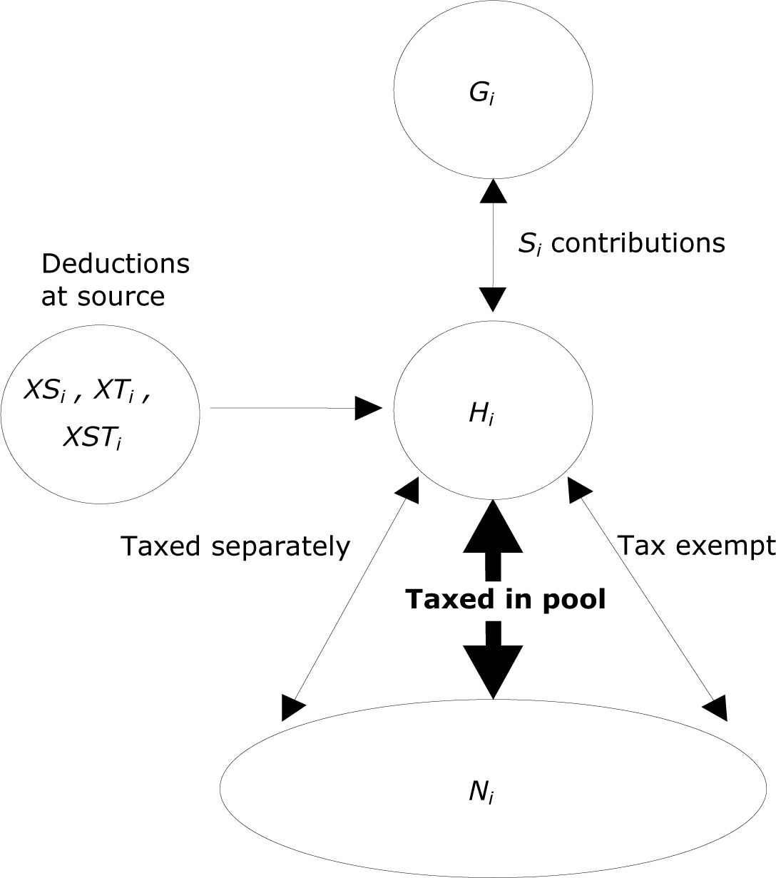
Basic relationship between net and gross amounts.
2. The basic gross-to-net conversion algorithm of SM2
Figure 1 shows the basic relationship between gross and net forms of income when more than one income component and possibly more than one individual in the tax unit are involved. The relationships between gross taxable income for a particular component, Hi and quantities like gross income Gi and income after retentions at source XSTi are usually simple, dependent only on i, the income component concerned and determined independently of other components and other persons in the tax unit. The same applies to the relationship between Hi and net Ni for components which are taxed separately at a flat rate or a rate determined by the level of income from that component alone, and of course also for tax exempt components. Sometimes, dependence of the relationship on other sources of income may also be involved, but mostly these are simply in the form of upper limits which may apply to certain quantities pooled over more than one component.
Generally, however, all or most taxable income is pooled together over components and over persons in the tax units for the purpose of determining the amount of tax due. The relationship between Hi and Ni for components in the pool is more complex than shown above. In any case, going from known Hi to Ni is less problematic since the relationships (the tax rules) are a function of the former. These relationships are specified in more detail in Table 1. Going from given Ni to H, required iterative solutions, and are described in the next section. Entries in Table 1 have the following interpretation. The last two columns of the table define the various income measures in terms of measures defined in the preceding rows; those in the first column concern total income, in the second they concern income components.
2.1 Social insurance contributions
The social insurance contributions Si, if applicable to the component, are generally a function of the gross amount Gi, but in the case of employment income excluding the employer’s contribution (see note (b) tois specific to the component Table 1). The functional relationship Si(Gi) is specific to the component and the country. In SM2 this is specified (and ‘called’ as a subroutine in the application programs) separately from the common structure represented in Table 1. However, some more complex situations can be allowed for in the model while retaining its basic structure. Specifically, it can allow for the dependence of Si for any particular component i on any set of income components, i.e., a functional relationship of the form Si = Si(GI), where subscript I refers to any set of income components (normally including the particular i, of course). In the French system for instance, the pooled contributions for a number of components may be subject to a common maximum limit.
Gross-to-Net conversion algorithm.
| Income measure | Total | By component a | |
|---|---|---|---|
| 1 | GROSS b | G=ΣGi ← | Gi |
| 2 | Social Insurance contribution | Si = Si(Gi) | |
| 3 | GROSS TAXABLE | H=ΣHi ← | Hi = Gi − Si |
| 4 | Component-specific deductions | Di = Di(Hi) | |
| Aggregation over components and individuals in tax unit | |||
| 5 | TAXABLE INCOME | Y=Σyi ← | Yi = Hi − Di |
| 6 | Common deductions | D0 = D0(H) | |
| 7 | Taxable income (after deduction) | Y0 = Y − D0 | |
| 8 | Tax due (before credits) | W0 = W0(Y0) | |
| 9 | Common tax credits | C0 = C0(Y0) | |
| 10 | TAX DUE | W = W0 − C0 | |
| 11 | Component-specific tax credits | C = ΣCi ← | Ci = Ci(Yi) |
| 12 | TAX PAID | X = W − C | |
| 13 | TOTAL NET INCOME | N = H − X | |
| 14 | Tax rate (descriptive) | R0 = X/H | |
| 15 | TAX RATE = TAX DUE/ TAXABLE INCOME | R = W/Y | |
| Disaggregation – personal income by component | |||
| 16 | Proportionate tax by component | Xi = (R*Yi) – Ci | |
| 17 | NET INCOME BY COMPONENT | Ni = Hi – Xi | |
-
a
The functional relationships in this column may be somewhat more complex or varied.
-
b
Gross including employers’ social insurance contribution (SS) is: GG = G + SS(G1)
2.2 Deductions
(Net) taxable income (row 7 of Table 1) is obtained by subtracting from gross taxable income the part which is tax exempt (‘deductions’). These deductions are a function of gross taxable income and may be of two types: (i) specific deductions which apply to the particular income components Di (row 4); and (ii) common deductions which apply to the (remaining taxable) income from all sources together (row 6). In case (i), in most situations the functional relationship Di(Hi) is specific to the component i, i.e., Di depends on the gross taxable income Hi for the component concerned. As a generalisation, the model can allow for the dependence of Di for any particular component i on any set of income components, i.e., a functional relationship of the form Di = Di(HI); or even more generally as Di = Di(HI, GI), where subscript I refers to any set of income components (normally including the particular i, of course). In case (ii), a functional relationship of the form D0(H) is in terms of total gross taxable income i.e. all components together. Both types of functions are of course country-specific. Again, in SM2 these relationships can be specified separately from the common structure represented in the table.
2.3 Aggregation
After the removal of component-specific deductions, it is necessary to pool the income over individuals in the same tax unit and across components which are treated together for taxation purposes. Certain income components may be excluded from this common ‘pool’ and taxed separately; this type of situation is accommodated in the present model (see Section 4).
2.4 Tax credits
Initial tax due is computed as a function of total taxable income (row 8). This is determined by the country’s ‘basic’ income tax schedule, normally applied to pooled income from different sources. This tax liability is normally reduced by tax credits. Tax credits are mostly based on characteristics of the unit (single parent, pensioner, etc.) or are given in compensation for particular expenses (medical, educational, etc.), i.e., are not specific to a particular income source. We refer to these as ‘common tax credits’ (row 9); these are normally expressed as a function of the total taxable income. The result is a more precise expression of ‘total tax due’ (row 10). In addition to the common tax credits, there may also be component-specific tax credits (row 11). Generally, these are based on net taxable income for the component concerned. However, the functional relationship may be more complex, involving other components of income and/or income in other forms (gross, gross taxable, etc.).
2.5 Tax paid and net income
Deduction of these tax credits from the amount of tax due (as defined in row 10), gives the final tax to be paid (row 12): i.e., total tax to be actually paid is tax due, less all (common as well as component-specific) tax credits. Total net income is total gross taxable income less tax paid (row 13)1. The above two quantities, tax paid and net income (rows 12–13) refer at this stage to total income, and not to income by individual component.
2.6 Tax rate
This refers to the effective tax rate which applies to pooled components. Tax rate in Table 1 has been defined in two forms. (i) The first (row 14) is a descriptive measure. It is the ratio of the total amount of tax to be paid, to the total gross taxable income (row 12/row 3). Hence it is indicative of the overall tax burden. (ii) The second (row 15) provides a more analytical measure in the following sense. It is the ratio of the total amount of tax due before taking into account any component-specific tax credits (row 10), to the total taxable income after removing component-specific deduction (row 5). By removing all known component-specific aspects, that is component-specific deductions and tax credits, R can be seen as the common rate which applies to all taxable income, from whatever source, which has been pooled and is subject to a common tax schedule.
Parameter R has two functions. Firstly, it provides a means for the disaggregation of total tax and net income into components when required (see below). Secondly, it is the parameter of the iteration in going from net to gross, as described in the next section. The parameter is particularly useful when modelling in conjunction with imputation for missing data (see below).
2.7 Disaggregation of tax and net income by component
This common ‘tax rate’ can be seen as a rate applying to each component individually, and not merely some average rate applicable only at the level of total income. This permits the decomposition of tax paid by income components (row 16), and consequently the decomposition of total net income into components (row 17). This decomposition is essential for the construction of variables such as net income before and after social transfers. Generally such decomposition is required in less detail than the breakdown of gross income by individual component.
The table involves six country-specific relationships or tax schedules. Three concerning total income:
And another three specific to each component (i):
The functional dependence can be somewhat more complex than indicated above, as explained earlier. In addition, there may be parameters determining retentions at source, taxation of parts of social insurance contributions, and so on. Finally, it should be mentioned that the application of various formulae and relationships requires certain constraints to be met, such as to ensure that all quantities which, to be meaningful, must be non-negative are in fact so. It is not useful to list here such (and many other) programming details. The structure in Table 1 is very general and provides a common framework accommodating a wide variety of specific situations. We have tested this in the case at least of the four European countries (Italy, Spain, France and Greece) for which the fiscal systems by individual income component have been examined in some detail.
2.8 Tax rate for modelling in conjunction with imputation
The role of ‘analytical tax rate’ as defined above is even more important in the presence of missing data where modelling has to be used in conjunction with imputation. The problem is that, on the one hand, the available information on income is in heterogeneous forms, and on the other, some of this information is missing and needs to be imputed. This requires the use of imputation and modelling techniques in conjunction. The issue has been explored in a separate paper (Betti et al., 2003); here we summarise the main points.
Imputation refers to the process of using the information existing in a dataset, as well as external information where appropriate, to produce improved estimates for missing, implausible or inconsistent elements in the dataset. The aspect with which SM2 is concerned with involves modelling in the context of household and personal income data, meaning generating and relating detailed information on income, by source (component) and type in its different forms, according to ‘destination’, i.e. according to how gross income accrued by households and individuals is partitioned into taxes, social insurance contributions, and the remaining net amounts available for private consumption.
These two statistical processes of imputation and modelling have to be implemented in conjunction with each other – in so far as imputation must be based on ‘donor’ data in a homogeneous form (which is the function of microsimulation in the above sense to create), while microsimulation generally requires data with no missing values (which is the function of imputation to ensure).
Any good micro-level imputation procedure must meet some basic standards. The imputed values generated should preserve the correlation structure of the data, should be determined stochastically rather than deterministically, and should be consistent or at least plausible. There are added requirements when we are dealing with complex, composite variables such as survey information on household and personal incomes. To impute where possible and reasonable is more critical for this type of data: total household income is made up of a large number of components, and rejecting a unit with incomplete information is unacceptable as it would result in the loss of much valuable information. Income components as variables do not form an independent set: they are mere components of the same ‘organic’ aggregate (total income of the household), and hence it is not meaningful to impute individual components separately. Even how that aggregate is partitioned is not predetermined, and hence nor is the resulting correlation structure of the data.
Forms of reporting of an income component.
| Income component (i) subject to tax and social insurance contributions | |
| Form (Xi) in which data on the income component have been collected: | |
| Gi | gross income (before tax and social insurance contributions, if applicable) |
| Hi | gross taxable (before tax, but after social insurance contributions, if any) |
| Ni | net income (after deducing ‘final’ tax and social insurance contributions, i.e., as the final amount actually received) |
| Income received after retentions at source: | |
| XTi | taxed at source (but no social insurance contribution); Ti = tax at source |
| XSi | Social insurance contributions (but not tax) at source; Si = social insurance contributions at source |
| XTSi | both tax and social insurance contributions at source; Ti + Si |
3. The core iterative procedure: Net-to-gross conversion
The form in which data on income by component are available may vary from one country (tax regime) to another, and also among individuals and households within the same country. There are two dimensions of this variation:
(A) Whether and how a particular component is subject to social insurance contributions and to income tax. Income tax may apply in various forms. (i) Some components may be pooled together, across components and also across individuals in some appropriately defined tax unit. (ii) Some may be subject to tax separately, each at a certain flat rate. (iii) Some components in the ‘pool’ may be tax-exempt up to a certain flat rate but taxed beyond that if a higher rate applies. (iv) Some may be subject to double taxation, perhaps representing some combination of the other forms.2 (v) And of course, many types of incomes, in particular social transfers, may be tax exempt. Mostly, the form applicable to each type of income is determined by the national tax regime, normally uniform for all respondents in a country. Hence this information can be compiled at the aggregate level and need not be collected at the micro level. There can be exceptions, however, for persons in special circumstances. There can also be other complications, such as more than one components, otherwise treated separately, being subject to common ceilings. In some systems, individuals have a choice among the various options.
(B) The form in which the information has been collected. This may generally vary from one individual to another in the same survey, though a uniform reporting form for the whole sample may prevail for some components. In any case, the information on the form in which the data are available is required at the micro-level. The amount may for instance be reported as gross, or as net of social insurance contributions and/or tax. In the case of tax retentions, details may vary by, for example, whether they are ‘retentions at source’ according to some rules or depend on individual arrangements, and whether they are the ‘final retentions’ of the tax actually due.
Table 2 lists the various reporting forms.
In this section, we describe the standardised ‘core’ of the SM2 system, taking account of complexities of (B), but assuming for the moment that through the information may be reported in diverse forms, all income components over individuals in the tax unit are pooled together and subject to a common tax schedule. A remarkable feature of the system is that by appropriately defining certain ‘deductions’ and tax credits, much more complex variation can be incorporated into this standardised procedures; this will be explained in Section 4.
3.1 Income net of tax
As noted above, in the case of tax retentions, an important distinction is to be made between: (i) ‘retentions at source’ (withholding taxes), and (ii) the ‘final retentions’ as appropriate for the income source concerned. This is a very important distinction. It is essential to know what is meant when a component is reported as ‘net of tax’. Does the information on retentions refer to withholding taxes, to final taxes, or even to some mixture? In some systems the withholding tax is quite different in size as well as structure to the final tax liability, and the taxpayers may even be able to choose their withholding rate of tax.3
3.2 Tax retention at source
Among the two forms of tax deductions, this may be the more common form in which net income is reported. We take ‘retention at source’ to mean that the amount of tax has been assessed depending only on the income received from the particular source concerned, not taking into account income received from any other sources or the individual’s (the tax unit’s) personal characteristics.
Indeed, in many situations, these retentions may be according to relatively simple and standard rules, which may be expressed, say, as T = (Hi − XST) = Ti(Hi), where tax retention at source (T), being the difference between gross taxable income (H) and the amount received after social insurance and tax retention at source (XST), is some known function of gross taxable income for only the component concerned. Provided that these rules are standard and known, XST, is directly convertible to Hi without reference to other components of income for the unit. By comparison, the relationship with Hi of the ‘final net’ Ni is more complex, as it depends on the unit’s total income from all sources. The real difficulty however arises when the rules for retention at source are not standard, are not applied uniformly, or are even non-existent in the sense that the taxpayers can choose or negotiate their withholding tax rates. In such situations, the construction of the gross taxable amount from the reported amount after withholding tax will require separate information on the amount withheld (or the withholding rule applied) in the particular case.
Calculation of Hi according to the form in which the component is specified.
| Set H | |||
| given value Pi = | XSi | Hi = XSi | Simple iteration, generally separately for each component |
| Gi | Hi = Gi − Si(Gi) | ||
| XTi | Hi = Gi − Si(Gi) where Gi = XTi + Ti(Hi) | ||
| XTSi | Hi = XTSi + Ti(Hi) | ||
| Set N | |||
| given value Pi = | Ni | Hi = Yi + Di(Hi) where Yi = [Hi − Ni + Ci(Yi)] / R |
Double iteration (i) with assumed R, for each component in turn (ii) for determining R, common to all pooled components |
-
Set N: set of income components which are subject to income tax (irrespective of whether the component is also subject to social insurance contributions), and for which the ‘final net’ amount (Xi = Ni) has been specified in the data collected.
-
Set H: all other income component (not subject to tax, or for which the data has been collected in a form other than
3.3 Final tax retention
In contrast to the above, the final tax retention is meant to reflect the tax actually due after taking into account the total income situation and characteristics of the tax unit. Consequently, the rules involved in this case tend to be more complex and involve the nature of the unit (individual person, household, or some other tax unit), the unit’s particular circumstances, and its income from all sources simultaneously. On the other hand, those rules are supposed to be applied (except for tax evasion and similar factors not considered here) in a standard way, not subject to variations according to individual arrangements as may apply to some retentions at source.
In practice, there may often be some ambiguity as to what a figure reported as ‘net’ by a survey respondent actually represents. For instance, employers often adjust the employee’s ‘tax code’ on the basis of tax returns for previous years, such that the amount withheld at source actually approximates the amount of ‘final tax’ which the employee would have to pay on this income in accordance with the prevailing tax rules. In the presence of such ambiguity, it is perhaps safer to interpret the amount reported in the sense of ‘net after paying the final tax due’.
3.4 Social insurance contributions
In contrast to tax retentions, social insurance contributions are essentially component-specific, i.e. determined only or mainly in relation to the income component concerned, so that the above distinction between ‘retention at source’ and ‘final retention’ is generally not relevant. They are usually collected at source in any case.4
3.5 Conversion routines
Table 3 shows the procedure for converting the reported amount with any combinations of the above dimensions of variation into a standard form. As noted at the bottom of the table, the income components may be divided into two sets, N and H, depending on whether the amount reported is ‘final net’ (Ni), or is in some other form (Gi, XSi, XTi, XTSi, Hi) more directly convertible to the ‘gross taxable’ form Hi. For all forms other than ‘final net’ Ni, it is convenient to take ‘gross taxable income’ Hi as the standard target of the conversion:
This conversion involves the component and country-specific functional relationships or schedules, namely Si = Si(Gi), for social insurance contributions, and Ti = Ti(Hi), for tax retention at source.
As noted, tax retentions at source may be according to fixed schedules, or according to arrangements determined at the individual (micro) level. In a majority of the cases, Hi can be determined directly from the collected amount, for instance from gross amount (Gi) reported for an income component i subject to social insurance contributions, we have: Hi = Gi − Si(Gi). In other cases, an iterative procedure may be required. However, generally the iteration is very simple and converges quickly. This is because by and large component-specific schedules apply to each component separately. There are no other parameters to be estimated. The need for numerical iteration arises simply from the fact that the unknown quantity to be determined (Hi) appears in an implicit equation.
The second panel of Table 3 shows the relationship between Hi and the reported amount in the form ‘final net’ Ni. Going from Ni to Hi in fact involves a double iterative loop. The inner loop of iteration is applied with an assumed value of the parameter ‘tax rate’ (R, as defined in Table 1). Once this has been done for every income component in the group (including over all individuals in the same tax unit), an outer iterative loop obtains a convergent value of this parameter which is common to all those components. The Ni to Hi conversion process is therefore considerably more complex. Furthermore, this complexity is substantially increased in the presence of missing data, where the modelling and imputation procedures will have to be applied interactively.

Common structure of the iterative model.
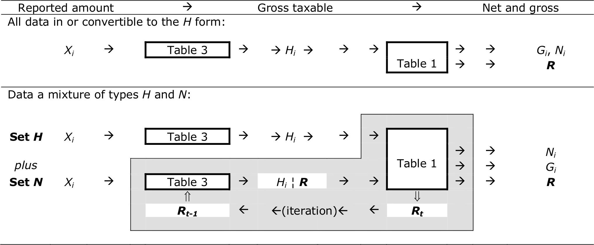
3.6 Iterative procedure
Table 4 demonstrates the common structure of the iterative procedure. The procedure distinguishes between sets H and N as defined in Table 3, and may be applied as follows. The required Hi quantities for set H are computed (only once) using Table 3, and form an input into the iterative cycle for parameter R required for set N. The parameter is best estimated by using information on all income components from both the sets.
The net-to-gross iterative procedure can be affected by two common problems in microsimulation modelling: non-convergence and multiple-convergence.
By non-convergence we mean that starting from a net value, the procedure is not able to find any gross value. This may be because no gross value exists as a result of some peculiarities of the data, tax-benefit rules, or hypotheses made concerning deductions or tax credits which cannot be calculated from available data or rules. Alternatively, this may happen when in principle a solution exists but the SAS routine does not converge to the solution in an ‘acceptable’ number of iterations. In SM2 SAS routines, this problem is dealt with as follows. The system finds a gross value the net corresponding to which is the closest to the given net value. Then the ratio (given / computed) net for each component is used to adjust its computed gross proportionately. The adjusted gross value can be taken to correspond to the given net amount. The adjustment required is usually very small.
For identifying the problem of multiple convergence, the SAS routine introduces small random perturbations in the computed ‘tax rate’ R in order to identify whether it is a ‘local convergence’, i.e. whether there exist multiple values of gross which correspond to exactly the same given net value. If the problem of multiple convergence is identified, some judgemental (‘reasonable’) criteria have to be used to select a particular solution.
4. Special deductions and tax credits: A device to treat diversity
A remarkable feature of SM2 is that by appropriately defining certain ‘special deductions’ and tax credits, many special features and complexities of different tax regimes can be incorporated into the standardised procedures described in the previous section without altering them in any way.
Deductions refer to the part of gross taxable income which is tax exempt. As noted, these deductions may be component-specific, or may be common deductions which apply to taxable income as a whole. Initial tax due is computed as a function of total net taxable income. This tax liability is normally reduced by tax credits. Again, these may be component-specific, or may be common credits which apply to the initial tax due as a whole. In addition to these ‘normal’ deductions and tax credits, we can define ‘special’ component-specific deductions and tax credits to accommodate variations in the form in which the component is taxed without altering any other aspect of model specification. Table 5 lists a number of such possibilities. In fact, it covers all the situations we have encountered in the diverse fiscal systems of various EU countries, notably those of France, Italy and Spain for which we have developed detailed applications of SM2.
Examples of special deductions and tax credits.
| Form of taxation of component i | Special deduction | Special tax credit | |
|---|---|---|---|
| 1 | Tax exempt | Di = Hi | − |
| 2 | Taxed at flat rate fi | Di = Hi | Ci = −fi × Hi |
| 3 | Tax-exempt at flat rate fi | − | Ci = +fi × Hi |
| 4 | Deductions for expenses | + common deductions | − |
| 5 | Tax credit for expenses | − | + common tax credits |
| 6 | Special tax not related to income | − | − common tax credits |
| 7 | Double taxation at flat rate fi | − | Ci = −fi × Hi |
| 8 | Part ΔSi of social insurance contributions subject to tax | −ΔSi | − |
-
Different forms may apply to cases like 3, 4 and 7: for instance the tax rate being a more general function of the amount of income involved for the component concerned.
Consider for instance the common situation with one component (such as family benefits) tax exempt, and the remaining components pooled together and subject to a common tax regime (row 1 of Table 5). By simply specifying ‘special deduction’ for the tax exempt component as Di = Hi, i.e. the same as its gross taxable amount, we automatically retain its tax-exempt nature and it is no more necessary to separate it from rest of the pool. It makes no contribution to the total net taxable income, and its original gross taxable income appears automatically as a part of the final net income. Similarly, if a component is taxed at a flat rate (say fi) separately from the pool (row 2), we can simply specify its ‘special deduction’ as Di = Hi, and its ‘special tax credit’ as a negative quantity Ci = –fi × Hi. It makes no contribution to the tax liability of the pool, but the final tax liability is automatically increased by the appropriate amount. Again, no other treatment separate from the pool is required for this component.
The situation in the case of a component tax-exempt at a flat rate is just the opposite (row 3). Deductions for expenses can be specified as common deductions applicable to the total income i. e. not associated with any specific income component (row 4), and similarly for tax credits for expenses (row 5). Sometimes components are subject to ‘double’ taxation. For example, in Italy self-employment income is liable to income tax as a part of the total income in the normal way, and also to an additional tax (‘IRAP’) at a rate depending only on the component concerned. This complexity is easily handled as shown in row 7.
The last case (row 8) is an important one, as it handles a special and complicating factor in the treatment of social insurance contributions, which themselves are subject to tax, as in France for instance. By specifying the taxable part of social insurance contributions as negative deductions from (i.e. in effect as additions to) gross taxable income (Hi = Gi − Si), the net taxable income (the amount actually subject to tax) is augmented by the taxable part of the social insurance contribution, say ΔSi: Yi = Hi + ΔSi. No further special treatment of this feature of the system is required in the model, despite the complexity and unusual nature of this feature.
5. A description of the italian fiscal system
By way of illustration, this section describes the use of the SM2 model to construction of EU-SILC target variables on income for elements of the Italian fiscal system, and implemented for the reference year 2003. Applications have also been developed for other countries. The essentials of the national systems in terms of main components of income, tax and social insurance contributions will be described below in Table 6 for Italy. Similar tables for Spain and France are provided in the appendix (Tables A.1 and A.2). There we also note briefly some features of these countries’ fiscal systems that appear particularly difficult to model in principle, but are handled in a relatively straightforward way within SM2 structure. See also comments in Section 4.
5.1 Income components
Table 6 summarises the main income components and shows whether or not they are liable to social insurance contributions and income tax in the Italian system. The table depicts the relationship between gross income, net income and the structure of the fiscal system.
Income from work (employment and self-employment) is subject to social insurance contributions, determined as a function of gross income (Gi). These contributions are subtracted from gross income to obtain the gross taxable income. Social insurance contributions are not liable to income taxation, IRPEF. The only exception is the non-compulsory social insurance, which is taxed.
The main Italian income tax (IRPEF) is computed by applying marginal progressive rates to increasing income brackets. Most types of income are pooled together for this purpose. Self-Employment income is additionally subject to a special tax IRAP, determined as a function of gross taxable income from self-employment. As explained in Section 4, such ‘double taxation’ is handled in our model by simply treating it as a ‘negative tax credit’; it is for this reason that this additional tax on self-employment income is shown in the last column of the table under ‘component-specific tax credits’.
Main components of income, and tax and social insurance deductions in the Italian fiscal system (year 2003).
| N | Income Components | Social Insurance Contributions (Si) | Tax | Included in common pool | Component-specific | |
|---|---|---|---|---|---|---|
| Deduction (Di) | Tax Credits (Ci)c | |||||
| 1 | Employment income | Employer’s S0(G1) Employer’s S0(G1) |
IRPEF a | X | D1(Y1) | |
| 2 | Self-employment income | S2(G2) | IRPEF | X | D2(Y2) | −f2(H2) IRAP d |
| 3 | Pensions | IRPEF | X | D3(Y3) | ||
| 4 | Non-financial capital income | IRPEF | X | |||
| 5 | Property (rental and cadastral) income | IRPEF c | X | |||
| 6 | Financial Capital income | Taxed at source (flat rate K6) | H6 | −K6 × H6 | ||
| Education related benefits, Unemployment benefits | IRPEF | X | ||||
| 7 | Family benefits, Sickness invalidity benefits d, Housing allowances, Any other personal benefits. | Tax exempt | H7 | |||
| Assets | ||||||
| 8 | Property value | ICI (on value of real estate) | −f8(value) | |||
-
a
Above a certain limit and if it not taxed at source
-
b
Additional tax on self-employment income (IRAP, Tax on income from production activities). f(..) stands for "a function of"
-
c
On total cadastral and on 85% of the rental income
-
d
Part of the benefits may be taxable
Financial capital income is not subject to IRPEF but is taxed at source at a flat rate, which can again be specified as a negative ‘component- specific tax credit’ in our model. Special tax on property assets is handled in a similar way. Components which are not subject to the common IRPEF are removed from the common pool by simply specifying their ‘component-specific deductions’ as equal to the component’s total gross taxable income (so that their resulting contribution to net taxable income is automatically zero). This applies to financial capital income and to tax-exempt benefits.
A brief description of the different kind of income follows.
The employment income (wages and salaries) is earned by dependent workers – it is liable to social insurance contributions (paid both by the employers and the employee) and to income taxation, IRPEF. The self employment income is earned by non-dependent workers – it is liable to social insurance contributions and income taxation, IRPEF. Pensions are treated in the same way as the employees’ income, but they are liable only to income taxation (IRPEF) and not to social insurance contributions. The non-Financial Capital Income includes share dividends, and is liable to income taxation (IRPEF). The property income includes income earned from the possession of lands and buildings which are registered in the cadastral register. It is made up of rental and cadastral income. The tax base includes imputed income from owner occupied housing, income from letting or sub-letting, and other income from real estate property. Of rental income 85% is liable to IRPEF. When real estate property does not produce rental income, it is still taxed as cadastral income. Financial capital income includes mortgage, interest on deposits and accounts, bonds yields, complementary income from pensions and insurance, etc. It is subject to tax withholding at source at some flat rate.
Education related benefits are liable to income taxation IRPEF, the only exception are the university grants. They are not liable to social insurance contribution. Unemployment benefits are treated like employee’s income, they are liable to income taxation, IRPEF but not to social insurance contribution. Family benefits are not liable to social insurance contribution or income taxation. Family allowance is given to the head of the household provided that he/she is a dependent worker or pensioner and that wage or pension earnings are the main component (greater than 70%) of the total household taxable income. Their amount varies according to the level and composition of household income, and according to the presence or not of both parents. Housing allowances and any other personal benefits are not liable to social insurance contribution or income taxation. Sickness invalidity benefits are not liable to social insurance contribution but can be liable to income taxation. It depends on the institution which allocates them. If the disability is due to a work accident, the benefit is paid out by INAIL (Italian Workers’ Compensation Authority) and it is not liable to taxation. Otherwise the pension is paid by INPS (National Institute of Social Security) and it is liable to IRPEF. Finally, the property value is based on the cadastral value of the real estate. It is liable to a tax on wealth called ICI (Local Property Tax). In the SM2 incomes that are not considered in the income taxation are severance pay, income from main house, arrears subject to separate taxation, and the amount of pension needed to top-up a certain threshold.
5.2 Social security contributions
Social insurance contributions on income from employment and self-employment in the Italian fiscal system are determined taking into account many different characteristics of the individual and the family and work situation. It is not possible (nor useful) to enumerate those details in this paper, except to note a few salient points. These details are of course taken into account in the ‘country-specific’ routines of SM2 to the maximum extent possible, limited only by the type of information available for Italy in the data source such as ECHP or EU-SILC.
Since the incidence of contributions on earned income is different according to the type of income, occupational status and sector of activity, the model identifies their different characteristics. Employers’ and employees’ social insurance contributions are levied on gross earnings from wages5. For dependent workers there is a minimum and maximum amount of contribution to be paid. These two limits do not depend on earned income, but depend on firm size, sector of activity and occupational status. The social insurance contribution to be paid for self-employed workers is divided into three categories: that for general self-employed (i.e. craftsmen or workers in commerce), agricultural self-employed, and professional persons. The social insurance contribution rates are different in these categories and depend also on the age of the worker. There is also a common minimum and maximum base of contribution.
A special category of status in employment needs to be taken into account in Italy. This is the status of the ‘co-ordinated and continuative collaborator’, CoCoCo. This status, intermediate between dependent and independent employment, is likely to increase in importance in Italy. Actually the CoCoCo are self-employed, but because of their particular treatment in the Italian fiscal system, their position is not clear. The income produced by these collaborators is treated as employee’s income and, for this reason, the social insurance contributions are also paid by the employer. These contributions are, however, much lower than the normal ones for employees.
5.3 Deductible expenses
In the SM2 net taxable income is obtained by subtracting from gross taxable income some deductible expenses: some medical expenses; alimony; donations to religious institutions; and so on.
There is no survey information on these deductible expenses, which vary from household to household according to preferences and medical conditions. In order to have actual deduction values, Euromod Country Report on Italy (Euromod, 2004, Table 19), has been used in SM2 to provide an empirical basis for estimating the deduction rate as a parametric function of the logarithm of the income.
5.4 Tax units
In the Italian fiscal system taxation is levied at individual level or at the level of family nucleus. In particular, we have the following two types of tax units in a household:
Family Unit - includes the head of household and all dependent persons. The essential condition defining members of the household as dependent is that their income does not exceed a certain threshold. The income considered for tax purposes is only the income of the head of household; any income received by dependent persons is effectively tax exempt (i.e., is not pooled with that of the head of household for the purpose of tax assessment).
Individuals – who are part of the family, who are not dependent persons and declare their income separately. Each such person forms a separate tax unit.
The income of the Family Unit is the base for the calculation of the incidence of deductions and the eligibility for tax credits and family allowance. For all other persons who are members of the household but are not dependents, deductions and benefits apply at the individual level since they are taxed separately.
5.5 Income taxation
The main Italian income tax is IRPEF (Tax on Income of Individuals). There is no obligation to fill in the tax return under certain conditions. In any case, a person is obliged to make a tax return if he/she wants to claim deductions, tax credits or rebate of taxes already paid (at source or the previous year). The amount of gross income tax is determined by summing up IRPEF, Additional Regional IRPEF and Additional Municipal IRPEF. All residents who receive income, even if not in Italy, are subjected to IRPEF. The IRPEF tax is obtained by applying marginal progressive rates to the increasing income brackets. There are some typologies of income that, because of their characteristics of being either lump sum (una tantum) or of a special nature (concerning more than one fiscal year), are not subjected to income taxation (IRPEF) but to a different type of tax. An example is severance pay.
Capital income is composed of four different categories: dividends from shares, interest on bank account and other short-term investments, interest on private or government bonds, and gains on time contracts. All these categories are taxed in different ways. The IRAP represents tax on productive activity collected at a regional level. It is the main regional tax, and the first important example of administrative devolution in the Italian system. The IRAP tax is calculated as a percentage of self-employment income according to the typology of productive activities. In effect, IRAP amounts to ‘double taxation’ on self-employment income, which is also subject to IRPEF.
5.6 Tax credits
Tax credits are subtracted from gross income tax to obtain the value of net income tax to be paid. In the Italian fiscal system, there are different kinds of tax credits, some general ones depending on the household composition (tax credit for dependent spouse, children, and other dependent persons), and other component-specific depending on the income received (tax credit for dependent workers, pensioners and self-employed). In Italy some tax credits are also based on consumption expenditure on several categories of goods (e.g. medical expenses). In order to estimate those tax credits, information on the level and composition of consumption of households is needed. It has been necessary to use external sources to obtain such information.
6. The development of italy SM2-EU-SILC
In Italy the new EU-SILC survey was conducted for the first time in 2004: 24,270 households and 61,542 individuals were interviewed. The new survey replaced the ECHP (European Community Households Panel) survey as the main reference source at EU level for comparative statistics on income distribution and social exclusion.
For the net-gross conversion of EU-SILC income target variables, ISTAT decided to test the application of the SM2 model using the new survey data and to experiment with some methodological innovations based on the ISTAT experience in using both administrative data and sample survey data. The development of the SM2-EU-SILC for Italy required through revision and update of the existing ECHP-based SM2, developed by Verma, Betti and co-researchers as reported in Eurostat (2004). For one thing, EU-SILC collects additional relevant variables, and the model had to be extended to incorporate them.
Particular attention has been paid in the construction of the tax units for the estimation of tax credits for dependent persons. The tax credits for dependent relatives establish a connection between the household members; as mentioned previously, two types of tax units can be found in a household – a ‘family unit’ and the ‘individual’. To identify these two types of tax units at the household level, the ‘family procedure’ used in ISTAT social surveys was applied. The procedure allows the construction of family relationships in the households the identification of dependent persons.
6.1 Implementation of italy SM2-EU-SILC
The quality of the microsimulation results and their international comparability depend on the detail of the tax system incorporated in the model, and above all on the quality of input data. The production of net and gross income microdata derived from the same sample survey is an important innovation for Italy. Two aspects contributed to the new EU-SILC-based application being a major enhancement of the previous ECHP- based SM2.
Data improvement:
a better estimation of social security contribution of CoCoCo (co-ordinated and continuative collaborators);
a wider range of available data, for example concerning pension contributions to private entities, sickness and invalidity benefits, local property tax (ICI), etc;
Methodological improvement:
tax credits and deductions estimated from tax returns instead of imputations;
possibilities of comparison of microsimulation results with administrative data.
Since in Italy both survey and tax data are used for the estimation of employee income, selfemployed income and old age benefits for the EU-SILC target variables, administrative data are used as inputs to SM2 as exogenous information on tax credits and deductions. The calculation of income deductions and tax credits is based on consumption expenditure and the available administrative data derived from tax returns. Two relevant data sets are used for the record linkage: the ‘UNICO tax returns’ used by all the taxpayers and in particular by self-employed workers, and the ‘730 tax returns’ used by employees and pensioners. Through an exact matching of administrative and survey records, the two tax data sets are integrated with survey microdata so as to construct the needed income deduction and tax credit variables.
This combined use of tax and survey data represents the most important methodological improvement in the SM2 implementation for Italy. Administrative data are used in the input file of the model instead of estimation by regression technique based on external sources. Moreover, the linkage with administrative data permits validation of microsimulation results. Of course, some problems can be expected in using tax and income data from administrative sources. The definition of taxable income or tax units in administrative sources can be different from that in surveys. In addition, the tax data derived from individual tax returns generally have an incomplete coverage of non-taxable income. Of course, register data cannot take account of tax evasion and tax avoidance. Some additional problems of inconsistency between survey and tax data can also be foreseen.
In the case of Italy, combined use of tax and survey data seems by far to be the best approach. Using only the sample survey income in the microsimulation model is likely to involve an underestimation of gross and net incomes, and of taxes. Using only the tax data would involve a possible mismatch of income definitions and the problem of incomplete coverage of income, including as a result of tax evasion. Using both tax and survey microdata for the microsimulation has the advantage of reciprocal comparison and validation of data. Some problems could come up when income is reported in only one data source, and when the net survey income is larger than the gross tax income in tax records. The handling of these problems will be a priority objective in the further development of SM2 EU-SILC application for Italy.
EU-SILC target variables: distribution of income by component.
| Ratio net/gross | ||
|---|---|---|
| 6.1.1.1.1.1 | Income from work | 64.5 |
| PY010 | employee cash or near cash income | 85.9 |
| employer’s SI contribution | ||
| employee’s SI contribution | ||
| PY050 | cash benefits or losses from self-employment | 76.3 |
| Self-employed SI contribution | ||
| 6.1.1.1.1.2 | Property income | 80.7 |
| HY090 | interest, dividends, profit from capital investments in unincorporated business | 81.1 |
| HY040 | income from rental of a property or land | 80.2 |
| 6.1.1.1.1.3 | Taxable benefits | 88.6 |
| PY090 | unemployment benefits | 92.5 |
| PY100 | old-age benefits | 88.7 |
| PY110 | survivor’ benefits | 87.9 |
| PY130 | disability benefits | 90.2 |
| 6.1.1.1.1.4 | Tax-exempt social transfers | 100.0 |
| PY140 | education-related allowances | 100.0 |
| HY050 | family related allowances | 100.0 |
| HY060 | social assistance | 100.0 |
| HY070 | housing allowances | 100.0 |
| HY080 | regular inter-household cash transfer received | 100.0 |
| Total | 71.3 |
At this stage, Italy SM2 should be considered as a work in progress. The next steps should introduce into the model procedures for the calculation of severance pay and the local property tax (ICI), which are not available in the application so far. The model should also account for the tax relief or the preferential tax regime that grants special benefits to some categories of employers (e.g. those with businesses in particular disadvantaged areas), and also improve the estimation of taxation on capital income of different types.
6.2 Results of the SM2 model
The SM2 SAS routines for Italy have been used for all individuals or tax units receiving non-zero income during the calendar year 2003. Most income components, collected as net (N) or taxed at source (X), have been converted into taxable income form (H) and to gross form (G) through the simulation of social insurance contributions. All EU-SILC income target variables can be constructed on the basis of appropriate aggregation of such classification by component.
Table 7 shows the main EU-SILC target variables. Actually, the model provides a breakdown for gross income, net income and the net-to-gross ratio, though all of these are not included in the required target variables in EU-SILC. Because of differences in component-specific deductions and tax credits, and also in the social insurance contributions, the net/gross ratio varies by component.
The net-to-gross ratio is much lower for income from work (64.5%) than for other components. This results from the social insurance contributions to which such income is subject. Leaving aside the effect of social insurance contributions, the ratio of net-to-gross taxable income varies approximately from the low of 80.7% for property income, to 85.9% for work income, to 92.5% for various taxable benefits, and of course to 100% for housing, social assistance and other tax-exempt benefits. These results appear plausible, though external data are not at hand to validate the breakdown in detail by component.
Table 8 shows the breakdown of total gross income into total net, social insurance, and tax amounts. According to SM2 estimates, net income, after tax and social insurance contributions including employers’ contributions, accounts for 71.3% of total gross. The table also shows comparison with figures published by ISTAT. The agreement is very good (with less than one percentage point difference in the net/gross ratio for the two sources); the SM2 can indeed be considered very satisfactory. Employers’ social insurance contributions are a little underestimated in SM2 compared with the ISTAT figures, while taxes and employee and selfemployed contributions are somewhat overestimated.
7. Concluding remarks
The Siena Microsimulation Model (SM2) has been developed to meet a very practical need in a systematic and efficient manner. In interview surveys collecting information on household and personal income, the respondents may report income amounts as gross or net of taxes and other deductions. The data must be made homogenous before use for analysis, especially comparisons across population groups and countries. SM2 provides a robust and convenient procedure for this purpose. Starting from data on household and personal income given in different forms, and on the basis of the prevailing tax regime in a country, the SAS routines of the model are designed to estimate full information on income by component, with a breakdown of gross amounts into taxes, social insurance contributions of various types, and net income.
There are at least three main ‘clients’ or potential users of this model.
Comparison with external sources: distribution of total gross income.
| SM2 | ISTAT | Error (% point) | |
|---|---|---|---|
| Gross including SI | 100.0 | 100.0 | |
| SI contributions | 15.9 | 15.7 | 0.2 |
| − Employers’ contribution | 9.9 | 11.4 | −1.5 |
| − Employees’ contribution | 3.5 | 2.8 | 0.7 |
| − Self -employment contribution | 2.5 | 1.6 | 0.9 |
| Gross taxable | 84.1 | 84.3 | −0.2 |
| Personal income tax and financial tax | 12.8 | 12.0 | 0.8 |
| Net income | 71.3 | 72.2 | −0.9 |
-
Sources: ISTAT: National Accounts (2003); SM2: Model run using Italy EU SILC Wave 1 (2003) as input
First potential users are the more general microsimulation models. Such models are widely used as an integral part of the policy-making process in tax and social policy areas, and over the past three decades, microsimulation has moved from the description of the distributional impact of the existing tax and transfer systems to a more complex tool for assessing the different impact of alternatives proposal for changing existing systems. The primary objective of these models is to provide, on the basis of specific micro-datasets incorporated into the system, a comprehensive facility for simulation of the effect of varying parameters of the tax-benefit system on the disposable income received by various segments of the population. Simulation of taxes and benefits under different regimes (fiscal policy options) also forms an output of the system. Such models involving tax-benefit simulation require very detailed and standardised information on household and personal income by component. The logic of such modelling essentially requires household income components in the gross form as inputs which are used to produce corresponding net amounts under the assumed tax-benefit system as outputs. In practice, however, generally the required input data are not available in a homogeneous gross form, especially when they come from interview surveys. The required data transformation can of course be done on an ad hoc basis, but it is more efficient, convenient and comparable to develop systematic procedures and tools for the purpose.
Consequently, given its specific purpose of estimating full information on income by component in both gross and net forms from empirical data, SM2 is not meant to be an alternative to general tax-benefit simulation models, but as a complementary tool which those models can usefully exploit. Of course SM2 itself is a microsimulation model. However, the microsimulation involved in SM2 has certain special aspects, which make SM2 somewhat unique. On the one hand, it is limited to a fixed tax-benefit regime – the one that actually exists, under which the available income amounts in different forms have been generated. On the other hand, it does not expect inputs in a homogeneous form but generates income amounts in both gross and net forms as outputs.
The need for gross-net transformation of course goes well beyond the specific context of microsimulation modelling. The second important clients of the model are Eurostat and the countries participating in EU Statistics on Income and Living Conditions (EU-SILC) project. As noted, the immediate context for the development of SM2 has been certain specific requirements of EU-SILC. The need arises from the fact that, while the source, type and form of input information varies across and even within countries, the output required at the European level has to be comparable and standardised. The information which can be collected is limited to particular forms because of limitations of the sources providing it. For instance in some countries, especially those with income registers, all income components are available in the gross forms; by contrast in many other countries, in particular in southern Europe, generally net received amounts only can be provided by the survey respondents. However, the information is required as a standard set of ‘target variables’ involving both gross and net forms from all countries participating in EU-SILC. SM2 is specifically designed to meet this requirement. Furthermore, the model has flexibility to deal with an annual flux of data in different forms across and within countries and also with periodic changes in the national tax systems, which a longitudinal data source such as EU-SILC must deal with. Hitherto, SM2 has been implemented for constructing EU-SILC target variables by National Statistical Institutes of Greece and, as described in this paper, Italy; moreover, Portugal (Rodrigues, 2007) and Spain have utilised procedures on the lines of SM2 (in the sense of using aspects of the SM2 logic and structure but developing country-specific software for implementation). Earlier, implementations using ECHP data were developed for Italy, France and Spain. It can be expected that, with the EU countries having to deliver to Eurostat microdata on household income components in the standard gross form (which became mandatory from 2007, EU-SILC wave 4), the need and opportunities for the use of SM2 are likely to expand further. Moreover, EU-SILC data are becoming available to a very wide body of researchers, including those engaged in tax-benefit simulations. Some of those may wish to use SM2 independently to generate more complete series of household income components in net and gross forms.
Hence the third important client of SM2 is international comparative social research, whether for policy or academic purposes. Diverse academic and policy research may require income components in both net and gross forms in greater detail. As emphasised in this paper, SM2 is designed at the outset for multi-country application, as a flexible tool which is portable to the maximum extent possible across countries despite great differences in fiscal systems. As noted in Section 4, a distinguishing feature of SM2 is that it can handle diverse tax-benefit regimes using a common logic and a standard set of procedures making it particularly useful for multicountry comparative application.6 Reflecting this, the system is designed such that its core consists of a standardised set of routines which can handle a great diversity of input data forms and national tax systems. Country-specific routines are required to specify parameters of the national tax system in an appropriately standardised form; they also standardise the input data format. These, then, form inputs to the central core of the system designed to generate the required standardised outputs. The system has been developed to maintain a clear distinction between the common and the country-specific parts, and even more importantly, to maximise the part which can be standardised. This feature makes the system an appropriate and convenient tool for multi-country application.
As an illustration of all these three aspects appearing in conjunction, let us consider in conclusion the potential use of SM2 for Euromod already referred to. At European level, the increasing need for cross-country comparison has led to the development of Euromod, an integrated multi-country model for the European Union implemented by a consortium of teams in 15 countries (currently being extended to 4 of the New Member States) for policy simulation. Euromod is a static tax-benefit microsimulation model that provides estimates of the distributional effects of national or European level changes in social and fiscal policy. EU-SILC now forms the reference source for Euromod at European level. Before the introduction of this reference, microdata from different sources were used, requiring a lot of efforts for harmonising national sources and for transforming available data into the required model database. One of the main advantage of using EU-SILC is that it potentially provides the microdata for policy simulation for all EU and closely related countries, and does so with increased comparability across countries (Figari et al., 2007).7 In order to maintain and even enhance this comparability, it is highly desirable that uniform net-to-gross conversion procedures are followed, and if possible to even avoid country-specific development of net-to gross conversion procedures. Clearly, the development and implementation of SM2 for countries where necessary would help in the harmonisation of the conversion procedures, with advantages for national EU-SILC data bases, for tax-benefit modelling such as in the context of Euromod, and for the wider requirements of inter-country comparative research. An added but not-always-obvious practical advantage is that often it would be easier for individual countries to adapt and complete SM2 application than to develop their country-specific net-to-gross conversion procedures ad hoc.
Footnotes
1.
Strictly, this may be referred to as ‘disposable income’. Sometimes the term ‘net income’ is used for gross income less social insurance contributions and tax due, while ‘disposable’ also takes into account inter-household and some other transfers.
2.
A unique example is provided by the French system, where a part of social insurance contributions (themselves akin to a ‘tax’) is subject to income tax.
3.
By contrast, there can also be systems (such as in Spain) which aim at fine-tuning deductions at source to match closely the final amounts due.
4.
The situation can be more complicated. However, generally such complications merely make the algorithm specifying the various functional relationships more elaborate, but there is no problem in handling them within the common structure of the model.
5.
‘Gross earnings’ are defined to be inclusive of employees’ social insurance contributions, but do not include the employers’ contributions. The latter are a function of gross earnings so defined.
6.
This is perhaps the feature of SM2 contributing most towards its uniqueness.
7.
Nevertheless Euromod has particular data requirements that are common across countries and others that are specific to national tax-benefit systems and an harmonised data source such as EU-SILC may have some limitations. Important restrictions, for example, are the level of aggregation of income variables within the household, instead of individual income or the aggregation of different type of income into harmonised categories (e.g. benefit incomes, housing costs).
Appendix
Main components of income, and tax and social insurance deductions: Spain (year 2003)
| Income component | ECHP/SILC variable | Social insurance contribution | Taxed at source | Tax-exempt | |
|---|---|---|---|---|---|
| 1 | Employees’ income | (PI1111/PY010), regular wage/salary earnings excluding lump-sum | Employers’ contribution f ; Employees contribution; Unemployment. Insurance. g | X a | |
| 2 | Unemployment benefits | (PI131/PY090) | X a | ||
| 3 | Pensions | (PI132/PY100 + PY110) includes old age and survivor’s benefits (2 EU-SILC variables) | X a | ||
| 4 | Family related benefits | (PI133/HY050) | X a | ||
| 5 | Sickness invalidity benefits | (PI134/PY120 + PY130) (2 EU-SILC variables) | X a | X b | |
| 6 | Other taxable personal benefits | (PI136/PY150) | X a | ||
| Flat rate taxed withholding | |||||
| 7 | Employees’ lump-sum income | (PI1112) | X c | ||
| 8 | Self-employment income | (PI112/PY050) | Self-employed social insurance | X d | |
| 9 | Capital income | includes both financial and non-financial capital income (PI121/HY090) | X d,e | ||
| 10 | income from renting out buildings or land | (PI122/HY040) | X d,e | ||
| Tax exempt | |||||
| 11 | Education related benefits | (PI135/PY140) | X | ||
| 12 | Housing benefits | (HI138/HY070) | X | ||
| 13 | Social assistance | (HI137/HY060) | X | ||
| 14 | Private transfer received | (PI123/HY080) | X | ||
-
a
All these components are taxed at source following the same rules as applied to employment income. The tax rate for deduction at source is determined on the basis of incomes from components 1–6, taken one at a time. By contrast, the final tax rate (IRPF) is determined on the basis of pooled income from all taxable components 1–10.
-
b
Some benefits in these categories are tax exempt, e.g. when the individual is completely disabled, or receive sickness benefit due to HIV
-
c
Taxed at source at the same rate as determined on the basis of (and applied to) employee’s income.
-
d
Taxed at source at a fixed (flat) rate, depending on the component concerned.
-
e
Certain (in particular non-financial) forms of capital income are not subject to withholding at source. Also special or local withholding rates apply to some forms. Similarly, only a part of rental income is subject to withholding. Assumption in the application using available data: As it was not possible to distinguish between different forms of capital income, in our application to ECHP data all capital income was treated in a uniform way as financial capital income.
-
f
Employee’s ‘gross income’ (including tax and social insurance contributions of the employee), plus employer’s social insurance contribution gives ‘labour cost’.
-
g
Assumption in the application using available data: It was assumed that unemployment insurance contributions are made by all employees, but only during the time they are in employment. In reality, not all persons in employment may make this contribution because it is not obligatory. On the other hand, persons may continue to make this contribution also during any periods of unemployment. Such variations are not available in data such as ECHP at the micro-level.
Main components of income, and tax and social insurance deductions: France (year 2003)
| Income from employment | |
| Total Cost of Labour | GG1 |
| Gross wages | G1 = GG1 − S0 |
| Wages Net of Social Insurance Contributions | H1 = G1 − S1 |
| Income net of social contributions | |
| Net Income | H − H8 a |
| Total Net Income | H |
| Tax base and tax | |
| Revenus Catégoriels | Yg = (H − Hs) + ΔS |
| Revenus Catégoriels Net | Yn = Yg − (D1 + D2 + D3 + D4) |
| Taxable Income | Y = Yn − (D5 + D6 + D7 + D0)b |
| (basis for Quotient Familial and Income Taxation) | |
| Quotient Familial | Q |
| Net Income taxes (IR) | X = Q × W(Y/Q) − (C + C0) |
| Income after tax | N′ = H − X |
| Disposable Income | N = N′ + H8 |
| Constructing the income components in SM2 | |
| Gross income (including employers’ SI contributions) | GG = G + S8 |
| Employers’ social insurance contributions | S8 |
| Gross income (excluding employers’ SI contributions) | Gi; G = ΣGi |
| Income component (i) | |
| 1. Employment income | |
| 2. Self-employment income | |
| 3. Pensions | |
| 4. Unemployment benefits | |
| 5. Invalidity benefits | |
| 6. Capital income ‘A’; Capital income ‘B’ (in fact all capital income treated as ‘A’) | |
| 7. Other incomes: including property and rental income | |
| 8. Benefits ‘A’; Benefits ‘B’ (in fact all benefits treated as ‘B’) | |
| Social insurance contributions (other than employers’) | Si; taxable part ΔSi |
| Gross taxable income | Hi = Gi − Si; H = ΣHi |
| Component-specific deductions | Di; D = ΣDi |
| Net taxable income | Yi = Hi − (Di − ΔSi) ; Y = ΣYi = H − D |
| Common deductions | D0; Y0 = Y − D0 |
| Common tax credits | C0 |
| Quotient Familial | Q |
| Tax due | W = Q × W0(Y0/Q) − C0 |
| Component-specific tax credits | Ci; C = ΣCi |
| Tax to be paid | X = W − C |
| Total net income | N = H − X |
| Net by component | Ni = Hi − [{Yi (W/Y)} − Ci] |
-
a
H8 are tax and social insurance (SI) exempt benefits; hence H8 = N8
-
b
D5 to D7 are in fact zero (no component-specific deductions)
References
-
1
Euromod and the Development of EU Social Policy. DIW Discussion Paper 467Berlin: DIW.
-
2
Tax Benefits Models. STICERD Occasional Paper, No. 10London: London School of Economics.
-
3
Statistical Imputation in Conjunction with Microsimulation of Income DataRivista Italiana di Economia, Demografia e Statistica 58:35–43.
-
4
Euromod: an integrated European benefits-tax model. Final Report, Euromod Working Paper EM9/01University of Essex: ISER.
-
5
Commission Regulation concerning EU-SILC as regards the list of primary target variables. EU-SILC 107/02Luxembourg: European Commission.
-
6
Euromod Country Report Italy (2001 Tax-Benefit System)Euromod Country Report Italy (2001 Tax-Benefit System), September, http://www.iser.essex.ac.uk/files/msu/emod/documentation/countries/italy/cr01it0904.pdf.
-
7
Income in EU-SILC: Net-Gross-Net Conversion; Common Structure of the Model; Model Description; and Application to ECHP Data for France, Italy and SpainEU-SILC 133/04, Working Group on Statistics on Income and Living Conditions (EU-SILC).
-
8
Using the EU-SILC for policy simulation: prospects, some limitations and some suggestionsComparative EU statistics on Income and Living Conditions: Issues and Challenges – Proceedings of the EU-SILC conference. pp. 345–373.
-
9
Dynamic microsimulation models: problems and prospects, Discussion paperLondon: STICERD, London School of Economics.
-
10
The Role of Survey Data in Microsimulation Models for Social Policy AnalysisLABOUR 11:83–112.
-
11
Microsimulation Modelling for Policy Analysis. Challenges and InnovationsCambridge: Cambridge University Press.
-
12
Statistics on income and living conditions model: net gross income conversion, Report to EurostatPireus: NSSG.
-
13
Income in EU-SILC – Net/Gross Techniques for Building and Using EU-SILC DatabasesComparative EU Statistics on Income and Living Conditions: Issues and Challenges. Proceedings of the EU-SILC conference.
-
14
Improving the Capacity and Usability of Euromod – Final Report. Euromod Working Paper EM4/08University of Essex: ISER.
-
15
Static microsimulation models in Europe: a survey. Discussion PaperUniversity of Cambridge.
-
16
Personal income in the gross and net forms: applications of the Siena Microsimulation Model (SM2)Universita degli Studi di Padova: Dipartimento di Scienze Statistiche.
-
17
Dynamic Microsimulation Models: A Review and Some Lessons for SAGE. SAGE Discussion Paper no. 2, SAGEDP/02London School of Economics.
Article and author information
Author details
Publication history
- Version of Record published: April 30, 2011 (version 1)
Copyright
© 2011, Betti et al.
This article is distributed under the terms of the Creative Commons Attribution License, which permits unrestricted use and redistribution provided that the original author and source are credited.