Simulating histories within dynamic microsimulation models
- Maastricht University / UNU-MERIT, The Netherlands
- Rural Economy and Development Programme, Teagasc, Ireland
- Article
- Figures and data
-
Jump to
- Abstract
- 1. Background
- 2. Base dataset issues in dynamic microsimulation
- 3. Data
- 4. Methodology I: modelling the histories
- 5. Methodology II: alignment and adjustment in the simulation
- 6. Results I: back simulating employment status
- 7. Results II: pension memberships and eligibilities
- 8. Results III: income variables
- 9. Conclusions
- Footnotes
- Appendix 1 Steps of Back Simulation
- Appendix 2 Estimates for Certain Retrospective Variables (Male)
- Appendix 3 Estimates for Certain Retrospective Variables (Female)
- Appendix 4 Estimates for Earnings
- References
- Article and author information
Abstract
Constructing a base dataset is one of the most important elements in the dynamic microsimulation modelling. However, the access to a long historical panel is usually restricted for many reasons. This paper aims to develop a back simulation method that has the potential to generate a consistent synthetic history panel based on a typical household survey dataset with some complementary statistics. The model uses Living in Ireland (LU) household survey as an example to reconstruct the individual labour market trajectory since 1939. The overall results of the simulated panel have been proven sensible and consistent based on several validation tests. This method opens the possibility to further investigate into several fields of application such as life-cycle income analysis and pension reform evaluation, which typically requires the historical profile of individuals and has traditionally been difficult to perform.
1. Background
Many countries today are facing the prospect of rapid demographic change in the decades ahead and numerous research papers have been devoted to the analysis of the implications of an ageing population. A number of microsimulation models have been developed to study this issue linked with social security, retirement incomes, and pension reforms. In order to generate an accurate and stable projection for elderly earnings and pensions, it is essential to include some historical information in the dataset, a luxury that many modellers do not have.
Microsimulation models are usually categorised as either “static” or “dynamic”. Static models, e.g. EUROMOD (Mantovani et al., 2007), are mostly arithmetic models that evaluate the immediate distributional impact upon individuals/households of possible policy changes, whilst Dynamic models, e.g. DESTINIE, PENSIM, SESIM (Bardaji et al., 2003; Curry, 1996; Flood, 2007), extend the static model by allowing individuals to change their characteristics as a result of endogenous factors within a model (O’Donoghue, 2001). Dynamic microsimulation models in theory, could offer more insights than static models as they usually integrate long-term projections and behaviour simulations; however, they are costly to develop and require a baseline dataset that is both rich in variables and historical information. These demanding requirements unfortunately are rarely matched by the existing data availability (Harding, 2007) and therefore compromises are often made in order to make the simulation possible.
This paper investigates longitudinal data availability issues in microsimulation and proposes a viable alternative by simulating a plausible and consistent history using a typical household survey panel from Ireland. The following section discusses the base dataset issues in dynamic microsimulation models and the potential alternatives. Section 3 describes the dataset used in the back simulation and Section 4 explains the modelling procedure of the back simulation, and followed by a description of the alignment technique used in Section 5. The three sections following report the results of the back simulation together with the validations, for employment status, pension memberships and earnings, respectively. A conclusion and discussion are provided in the final section of this paper.
2. Base dataset issues in dynamic microsimulation
2.1 Base dataset selection
Base dataset selection is important for a microsimulation model as the quality of the input data determines the quality of the output, yet this is not an easy task, as hardly any micro datasets contain all the information required by a dynamic microsimulation model that can be used to project the whole population. The difficulties of picking a base dataset have been discussed in several papers (Cassells et al., 2006; Zaidi & Scott, 2001). Typically, a dynamic microsimulation model starts with one or several of the following types of dataset:
Cross-sectional Household Survey Data
Cross-sectional Administrative data
Census Data
Panel Household Survey Data
Panel Administrative data
Panel data is generally preferred over crosssectional data as it records changes over time, a useful component in statistical modelling. Household survey data, e.g. EU-SILC data in EUROMOD (Figari & Sutherland, 2007), is frequently used as the basis of the base dataset, because it is rich in the number of variables of interests and offers information on the dynamics of behaviours. However, the time period in these survey datasets may be insufficient to provide certain historical information required for life-cycle modelling and analysis. Administrative data, although typically consisting of a more limited range of contextual variables, often provides a longer history and contains relatively high quality information for certain variables, e.g. tax, and in most cases, a higher number of observations. Some Scandinavian country models, e.g. the MOSART model in Norway (Fredriksen, 2003), are based on extensive and detailed register information. However, access to administrative records is typically fairly limited even from within a government.
For microsimulation models analysing the dynamics of elderly earnings or pensions, it is essential to have historical social economics variables that could be used to reconstruct the career trajectories of today’s elderly workers. This implies that an ideal dynamic microsimulation base dataset should contain the following information for each individual from birth:
Demographic information, which contains age, education, marriage, birth of children, household (or tax unit) formation and dissolution.
Employment trajectory information, which contains labour force participation records, historical earnings, types of job etc.
Pension membership and entitlement information, which contains the record of various pension schemes participation (including state, occupational, and private pension).
To meet these requirements a long panel dataset containing rich demographic, employment, and pension data is required; unfortunately, a dataset that matches the above description is not readily available to most researchers. Certain models (e.g. DYNASIM, CORSIM) as a result, have experimented with alternative methods such as statistical matching and simulation.
The first method, statistical matching, involves filling in the missing information required from a different but comparable dataset compiled within a similar time frame. For example, a microsimulation model based on a household survey dataset may need some historical earning records that are only available from another income study dataset. Under such a circumstance, a matching method may be used to fill in the information gaps based on a statistical model using available social economic characteristics shared by both datasets. The DYNASIM model was one of the pioneers in this area and uses Current Population Survey (CPS) as the base dataset matched with social security earnings records from administrative data. In DYNASIM3 (Favreault, 2004), the statistical matching was undertaken between two survey datasets, namely, Survey of Income and Program Participation (SIPP) and Panel Study of Income Dynamics (PSID), while PENSIM2 matches Family Resource Survey (FRS) and British Household Panel Survey (BHPS) to the Lifelong Labour Market Database (LLMDB) to incorporate household contextual data (Emmerson et al., 2004). In addition, statistical matching also occurs between survey and census datasets, e.g. SAGE matches survey data to their base census sample data to obtain the additional information required (Evandrou, 2004).
The second method used is to generate a synthetic historical panel using information from the base dataset itself. Unfortunately, the methodology of simulating histories is not as widely discussed as simulating future characteristics in the microsimulation field. There are many challenges in attempting to “back-cast” or “back simulate” historical earnings (and other characteristics) earlier in life (Harding, 2007). The DYNANCAN model uses a limited back simulation technique by imputing the historical earning profiles between 1966 and 1969 with limited retrospective consistency (Morrison, 1997;1998), whilst the CORSIM model simulates part of the historical profile based on a historical crosssectional dataset, matching the model output to historical aggregate information such as fertility and mortality rates (Caldwell, 1997). Nevertheless, the existing methods only impute the history for a limited number of years and they usually suffer from the inconsistency issues. While certain variables match the historical data at cross-sectional level, the longitudinal consistencies are typically ignored and variables covered are not extensive enough to support life cycle analyses and pension simulations.
There are advantages and disadvantages to both methods described above. Statistical matching can be used when there are sufficient matching variables in a comparable dataset and this method has the desirable feature of having a “real-world” value, although the quality of matching may vary substantially depending on the quality and quantity of matching variables. In some cases, certain variables, e.g. historical earning records, may not exist in any dataset or access is restricted due to legal restrictions. If these variables are needed within the model, then the only option available is simulation. Synthetic simulation has the advantage of flexibility but longitudinal consistency may be an issue due to the limited information available.
2.2 LIAM and its base dataset
LIAM is a dynamic microsimulation model designed to evaluate potential reforms of the Irish pensions system and other policies in terms of changes to life-cycle incomes, particularly on old age income replacement rates, poverty and inequality measures (O’Donoghue et al., 2009). Given the nature of the model, it requires a pension module which is able to simulate:
Life-cycle income distribution under a given pension system
Public and/or private pension fund accumulation and dissipation over individuals’ life-cycles, under a given pension system and alternatives
Effects of reforms of a given system on life-cycle income distribution, costs, and other redistributive measures
Since the model aims to evaluate the impact of policy change for those “at risk”, i.e. potential pensioners, an ideal historical panel would start in the year in which the oldest potential retiree in the dataset was born. However, one practical issue of alignment prevents generating meaningful values in the very early years when few individual exists in the dataset. As alignment is necessary to ensure the cross-sectional consistency with the historical values, it is necessary to keep a minimum number of the observations for each year that the alignment is applied. Therefore, the study sets the starting year of the historical panel in 1939, the year when the youngest retirees in 1994 (age 55) were born and the elder retirees in 1994 (age 75+) just entered the labour market for no more than a few years.
Furthermore, in order to simulate the potential pension income, it is necessary to include a set of important social economic variables, covering demography, employment, and pension information. These include:
Demographic data includes gender, age, marital status, number of children and education attainment
Employment data covers employment status (working or not), employment type (employee or self-employed), employment sector (public or private) and job income
Pension data includes the pension contribution to occupational pension and private pension, the fund size of the defined-contribution (DC) pension, and the type of pension claimed after retirement
LIAM ideally, should select a base dataset which has a long social economic history, i.e. a panel that looks like an extended version of the US PSID or certain administrative datasets available in Sweden/UK etc. Unfortunately, long historical panels do not exist for Ireland, neither in the form of survey datasets nor as administrative records, yet this missing information is crucial to life cycle modelling and analysis, as some forward simulation components, such as pension eligibilities, are built on the individual labour trajectory. Given these constraints, simulation is therefore the best tool for obtaining histories for LIAM. Compared with earlier works on the historical recreation in microsimulation model (e.g. CORSIM and DYNACAN), the model could reconstruct a much longer time period and focuses on the consistencies at both cross-sectional and longitudinal levels.
This paper, as part of the work developing LIAM, proposes a microsimulation algorithm which could generate a plausible, consistent and comprehensive historical panel based on a household survey dataset by extrapolating the retrospective variables concerning past employment history. Variables such as years of working and pension eligibilities are registered in the household survey and could be used to model a plausible working history for all individuals when taken together with information generated from some external statistics.
3. Data
This back simulation module is primarily modelled based on the 1994-2001 Living in Ireland Survey (LII) dataset along with some external statistics extracted from the pension questionnaire section of the 2002 Quarterly Household National Survey (QHNS), and the Irish census reports since 1930s.
The LII survey constitutes the Irish component of the European Community Household Panel (ECHP) and is a representative household panel survey that was conducted yearly on the Irish population between 1994 and 2001 (eight waves). The data contains panel information on demographics, employment, and other social economic characteristics for around 3,500 households in each wave. In 2000, an additional 1,500 households were brought into the dataset to compensate for the attrition since 1994. Table 1 lists some descriptive information of key demographic and employment variables in the LII dataset.
An overview of LII survey.
| Variable | Mean | Standard Deviation |
|---|---|---|
| Age | 34.15 | 21.86 |
| Gender | 0.50 | 0.50 |
| Married (%) | 38.91% | 0.49 |
| Average household size | 4.31 | 1.86 |
| Working population (%) | 38.18% | 0.49 |
| Public Sector worker (%) | 7.81% | 0.27 |
| Self-employed (%) | 7.73% | 0.27 |
| Retired (%) | 6.85% | 0.25 |
| Unemployed (%) | 5.40% | 0.23 |
| Percentage of the population with college education | 17.46% | 0.38 |
| Average reported years of work | 13.66 | 15.20 |
| Total number of household | 7,529 | |
| Total number of individuals | 23,955 | |
| Total number of observations | 100,639 | |
Besides the LII survey, the back simulation module also uses the information gathered from the QHNS survey, which is a nationwide household survey designed to produce quarterly labour force estimates in Ireland since 1997. In the first quarter of 2002, a special module dedicated to pension savings was added to the survey. QHNS is used in the back simulation mostly for alignments when estimating occupational and private pensions. Census reports prior to 1994 were used in the back simulation module in order to align certain important history aggregates.
3.1 Demographic base data
Demographic data is the foundation of a population-based simulation. The back simulation module extracts demographic information from the LII survey and surmises some data, for example the time of birth of each individual is calculated from age information in the survey and marriage status is derived from the reported age of marriage. In the case where a missing value is spotted, average data is used, e.g. it is assumed that an individual would get married at 25, the average age of marriage in Ireland in the1990s. Divorce and remarriage is not simulated for in the current history panel for complexity reasons, and education level is assumed constant once an individual has left the reported schooling period.
In the current version of the back simulation, cohorts that died before 1994 were not simulated, as the primary goal for the back simulation is to complete the career trajectory for the potential living pensioners. This simplification helps to reduce uncertainties within the history panel and lowers the modelling difficulties by avoiding potential complex interactions and consistency concerns of the synthetic population. One drawback of this simplification is that it raises the bar for alignment, as the simulated data will not be able to compare with the historical aggregate indicators. Fortunately, the Irish census data contains detailed information for each age gender subgroup. As a result, all alignments described in this paper can be performed at cohort level to ensure the consistency between simulated values and historical census data.
3.2 Exploiting the retrospective variable
The LIIretrospective variables provide information for survey contains certain retrospective questions similar to many household survey datasets. These questions are helpful in history recreation as they can pinpoint the time when certain events happened in an individual’s history, e.g. birth, marriage etc. In the LII survey, retrospective variables provide information for
the year when an individual started their current job and their job’s duration
the year when an individual first entered the labour market
the number of years spent in full-time education, employment (including selfemployment and farming), unemployment (seeking a job), illness or disability,
home caring or retirement duration since the age of 10
the duration of unemployment, if currently unemployed
While the information collected is highly relevant for back simulation, these retrospective variables may not contain high quality data. Missing values and inconsistencies are sometimes spotted across differing years of the LII survey, for example the declared number of years in school varying without engaging in education. This type of error could hamper the quality of the simulated histories severely, as there would be no reliable reference to constrain the shape of the career trajectory.
In order to mitigate the impact of lower quality data, it is useful to correct obvious mistakes in the data collection and impute the missing values to expand the base on the dataset. Adjustments are applied to enforce the consistencies with key variables (e.g. age) and avoid basic mistakes such as assigning college degrees to children. Since most retrospective values (more than 90% of the individuals) are not updated once collected in the base year, it is necessary to recalibrate the values from second wave onwards to ensure the consistencies with the recorded labour market activity in the previous year. For example, if the individual worked full time in 1994, the accumulated years of employment should increase by one in 1995. Same principle applies to other variables like years of education etc.
Table 2 presents an overall summary on the outcome of the retrospective variable adjustments and highlights the difference between the original data and the adjusted data in the base year (1994) when the retrospective data was first collected. This adjustment increases the usability of these variables by improving its internal consistency. The table does not include missing values, which are imputed in the next step.
Retrospective variables adjustment in the LII survey (base year).
| Sex | Variable Description | Original | Adjusted | Observations Adjusted (%) | ||
|---|---|---|---|---|---|---|
| Mean | s.d. | Mean | s.d. | |||
| Male | Years in full-time education or training | 6.83 | 2.67 | 6.67 | 2.85 | 2.28% |
| Years in employment, self-employment or farming | 19.38 | 17.88 | 19.32 | 17.88 | 0.40% | |
| Years in unemployment | 1.11 | 3.24 | 1.11 | 3.24 | 0.14% | |
| Years of illness/disabled | 0.39 | 2.88 | 0.39 | 2.88 | 0.02% | |
| Years spent on home duties | 0.21 | 3.30 | 0.14 | 2.63 | 0.23% | |
| Years in retirement | 1.01 | 3.44 | 1.00 | 3.42 | 0.07% | |
| Female | Years in full-time education or training | 6.92 | 2.36 | 6.77 | 2.57 | 2.23% |
| Years in employment, self-employment or farming | 9.17 | 10.68 | 9.10 | 10.64 | 0.51% | |
| Years in unemployment | 0.32 | 1.58 | 0.32 | 1.58 | 0.09% | |
| Years of illness/disabled | 0.27 | 2.39 | 0.25 | 2.26 | 0.05% | |
| Years spent on home duties | 12.76 | 17.21 | 12.70 | 17.14 | 0.17% | |
| Years in retirement | 0.34 | 2.43 | 0.33 | 2.39 | 0.05% | |
| Total | Years in full-time education or training | 6.87 | 2.52 | 6.72 | 2.71 | 2.26% |
| Years in employment, self-employment or farming | 14.29 | 15.59 | 14.22 | 15.58 | 0.45% | |
| Years in unemployment | 0.72 | 2.58 | 0.72 | 2.58 | 0.11% | |
| Years of illness/disabled | 0.33 | 2.65 | 0.32 | 2.59 | 0.03% | |
| Years spent on home duties | 6.48 | 13.88 | 6.41 | 13.77 | 0.20% | |
| Years in retirement | 0.68 | 3.00 | 0.67 | 2.97 | 0.06% | |
Missing values are imputed via a set of ordinary least squared (OLS) equations, where the number of years spent in certain employment conditions are estimated using a vector for personal characteristics. Imputed values are checked for consistencies with other variables like age, education and adjusted in case of conflicts.
Table 3 describes what variables are imputed using this specification and what personal characteristics are included in the vector. Models are separately estimated for males and females. Appendix 2 and 3 report the estimates obtained in the imputation equations.
Imputed variables.
| Imputed Variables | Personal Characteristics used (X) |
|---|---|
Years in full-time education or training Years in employment, self-employment or farming Years in unemployment Years of illness/disability Years spent on home duties Years in retirement |
Education, age, current employment status, chronic illness, retirement status, number of children in different age groups |
4. Methodology I: modelling the histories
This section describes the methodology used in the back simulation. While a back simulation model may use some historical information to refine the outcome, it also has a higher requirement on the output quality. Since the main purpose of this back simulation model is to recreate each individual career trajectory, it demands a high accuracy of the model prediction as the pension eligibility is highly sensitive to the past employment status. In a forward microsimulation model, one would typically use some kind of aggregated values (e.g. mean, standard deviation of the distribution) to evaluate the quality of the simulation. The predicted value does not need to be correct at the individual level as long as the distributions are reasonable. Nonetheless, in the case of backward simulation, one needs to ensure that the values are sensible at the individual level due to the longitudinal consistency requirement while maintaining the reasonable distribution shape at each crosssectional level.
Compared with a forward dynamic microsimulation model, a back simulation model could be more complex as it is designed to exploit more information both from historical values and retrospective information. In order to create a panel dataset that is as close as possible to the real history, three methodologies are used in back simulations:
Deterministic simulation
Semi-stochastic simulation
Stochastic simulation
The deterministic simulation generates the part of the history that is directly determined by retrospective variables and ensures that the generated history is perfectly consistent with the reported values. For instance, if an individual reports starting work at age 20, it is safe to assume that this individual was in work that particular year. The variables used in deterministic simulation include the age when an individual begins to work, the year in which an individual quit their previous job, the number of years spent in their current employment status (e.g. length of current job, unemployment etc.) and the number of years spent in each employment status.
Semi-stochastic simulation recreates certain historical events from retrospective variables in conjunction with some reasonable assumptions. While the deterministic simulation pinpoints the timing of some major events in history, it gives only incomplete information regarding employment trajectory. Semi-stochastic simulation is still largely based on the reported retrospective variables but might involve some assumptions. For instance, since most women take maternity leave when giving birth, it is reasonable to simulate a career profile interrupted in the year of childbirth with a high probability. Another example would be “back to work” social welfare benefit, which usually implies a period of unemployment for the years preceding claiming the benefit.
Stochastic simulation is designed to fill the parts of the history that cannot be inferred from deterministic and semi-stochastic processes and it recreates the history through the predictions of estimated econometric models with random components. This method is similar to a regular dynamic microsimulation model, such as DYNAMOD2 and SAGE (King et al., 1999; Zaidi, 2004), with the difference being that the back simulation model ages the population in a reversed direction and is subject to a much more restricted alignment procedure for consistency reasons. An outline of the simulation steps are provided in the Appendix 1.
4.1 Discrete variable simulation
Discrete variables include both binary variables, such as pension membership and categorical variables, such as job position. Since the pension, membership calculation only requires basic employment status and the technical issues in alignment, the current version of the back simulation only simulate binary variables. Binary variables such as employment status, pension membership etc. are modelled using logit models that produce a probability of an event occurring as the output. These binary variables could be modelled in the following generic form
Xi is the vector of personal characteristics. The error term can be decomposed into specific individual effects ui and an i.i.d. stochastic term v. While there are a few methods that can be adopted for controlling individual heterogeneity, this current version of the back simulation uses a simple logistic implementation for the program compatibility and the speed reason. Assuming that the stochastic term (vit) is i.i.d. with mean zero, the average of the error terms for each individual is an unbiased estimate for individual effects (ui). It then becomes possible to re-estimate the model using calculated individual effects and apply them to the simulation. Therefore, the final model applies can be described as
The method is essentially an adjusted “fixed-effects” logit model, which is a logit variation of the specification suggested by Mundlak (1978). It yields a higher predictive power as parts of the unobserved heterogeneities are modelled. Table 4 lists the variables included for each logit model. Models are estimated separately for male and females.
Components of the employment status equations.
| Equations | |||||
|---|---|---|---|---|---|
| Variables Included in the Equations | In-Work | Self-employment | Job Sector | Occupational Pension Membership | Private Pension Membership |
| Age or Age group | Yes | Yes | Yes | Yes | Yes |
| Age Squared | Yes | Yes | Yes | ||
| Age 65 or above | Yes | ||||
| Education | Yes | Yes | Yes | Yes | Yes |
| Gender | Yes | Yes | Yes | Yes | Yes |
| Work Experience | Yes | ||||
| Gave Birth to a Child in the current year | Yes | Yes | Yes | ||
| Work in the Public Sector or Not | Yes | Yes | |||
| Job Industry | Yes | Yes | |||
| Job Occupation | Yes | Yes | |||
| Lagged variables | Yes | Yes | Yes | Yes | Yes |
| Mean value of residuals | Yes | Yes | Yes | Yes | Yes |
4.2 Continuous variable simulation
Income yit is modelled as an extended Mincer type earning equation (Mincer & Jovanovic, 1981). It consists of a deterministic component (representing the dependence of income on current state variables), a random effect ui (to account for unobserved individual heterogeneity), and a stochastic component εit (which represents random variation over time, in addition to variation from state changes). The statistical form looks like:
Where Xi includes education attainment, labour market experience and unemployment experience in the equations. Earnings are estimated using a random effect specification and coefficients are reports in Appendix 4.
5. Methodology II: alignment and adjustment in the simulation
Alignment is a commonly used method for calibrating microsimulation models so that aggregate outputs from the model match the external projections or values. This is partially due to insufficient knowledge regarding microbehaviour to specify a fully dynamic model. Simulation models, if unbounded, may over or under predict the occurrence of a certain event, even in a well-specified discrete model (Duncan & Weeks, 2000). Therefore, although in theory alignment might be controversial (as a perfectly specified model with perfect data should not need any alignment), it is a de facto common practice for microsimulation models (see for example DYNACAN, CORSIM, and LIAM).
In the back simulation module, alignment shapes the earnings and the distribution of employment status in a way that is both consistent with historical census information and retrospective information. There are two types of alignments applied in this model; one is a cross-sectional alignment and the other a longitudinal alignment.
5.1 Cross-sectional alignment
Depending on whether the variable is continuous or discrete, the alignment technique applied is different. Continuous variables such as earnings were aligned to the same level for the first year of the survey in 1994 for each age, gender, and education group and wage growth was assumed to be equivalent to consumer price index (CPI) growth rate. The alignment is a proportional adjustment, which has been used in several models, e.g. Chénard (2000a, 2000b).
For binary variables such as employment status variables, the alignment matches the proportion of the population which has a certain employment status (e.g. working or not), to the external census values, or estimated historical values, for each age, sex and education group in a given year. The alignment is based on the probability predicted by the logit model, i.e. individuals with the highest predicted probabilities (with the stochastic term) would be selected. The method is described in details by O’Donoghue (2010).
One issue with the alignment usage in this particular study is the incomplete population. While the dataset is population representative between year 1994-2001, the lack of the deceased population makes the dataset biased in early years. To address this problem, cross sectional alignments are only applied at the sub population level, i.e. alignment by age, gender, education status etc. rather than at the whole population level.
5.2 Longitudinal alignment
Besides the cross-sectional alignment, the back simulation also requires consistency in the retrospective variables, which is crucial to the quality of the generated historical dataset, as one of the main purposes of a long panel dynamic microsimulation is life-cycle analysis (e.g. pension). Currently there are hardly any simulation models applying a longitudinal alignment, as most have been developed for forward simulation, where there is no benchmark with which to align the results. In the backsimulation module, longitudinal alignments are implemented for the following reasons:
The simulated life path should be consistent with the reported retrospective variables such as date of marriage, year when started working, education, childbirth etc.
The simulated number of years spent in a certain employment category (e.g. total years of work/unemployment) should be consistent with reported values in the LII dataset
The state, occupational and private pension eligibilities should be consistent with the simulated labour force trajectory
As discussed earlier, major life events are determined before the stochastic simulation to ensure consistency. The reported number of years spent within a certain employment category, as presented in the LII dataset, is taken into account during the cross-sectional alignment design process. Together with the deterministic simulation, it is possible to identify how many working years are left undetermined. Individuals without any “working years” left would be assigned as out of a job during the cross-sectional alignment procedure. Some small adjustments were applied after the panel was created to eliminate small gaps experienced during public sector employment.
The alignment for the state contributory pension eligibility is a bit more complicated. Ireland introduced a state pension system in 1953 and in order to be eligible for an Irish state pension, an individual has to contribute for at least 19.52% (10/52) of the time between their first eligible job and age 65. Self-employed jobs were not deemed eligible until 1988. Given this information, it is possible to influence the pension entitlement by modifying two factors within a career profile: the years of contribution and the density of contribution. For example, if an individual is not eligible for a state pension but the simulation gives an opposite result (a type I error), it is most likely that the model over-simulated the number of years worked with a pension eligible job, or that the starting year is too late. In this case, it is possible to improve the consistency by removing the years of working experience in eligible jobs and replace them with non-eligible activities. Meanwhile, a reverse correction procedure can be applied to type II error individuals (the ones with pension eligibility but without simulated eligibility).
A simplified case below demonstrates this algorithm (Table 5 and Table 6). Assuming there are three individuals in the dataset: A, B and C. They reported that they have worked 3, 4, 3 years in total in their lifetime respectively, and in 1994, B and C received state pensions. Based on the reported total years of work and the yearly aggregate alignment, the back simulation module may generate an output as below, where a black dot [•] means that an individual is working in that year and a white dot [°] indicates that the individual is out of work. As seen below, the simulation is able to reconstruct a history with a controlled yearly aggregate and consistent total years worked.
Simulated profile without adjustment.
| Year | 1950 | 1951 | 1952 | 1971 | 1972 | 1973 | Total Years of Work | Rate | Simulated Eligibility | Actual Eligibility |
|---|---|---|---|---|---|---|---|---|---|---|
| Individual A | ● | ○ | ● | ○ | ○ | ● | 3 | 33.3% | Yes | No |
| Individual B | ● | ○ | ● | ● | ○ | ● | 4 | 66.7% | Yes | Yes |
| Individual C | ● | ● | ● | ○ | ○ | ○ | 3 | 0.00% | No | Yes |
| Yearly Aggregate | 3 | 1 | 3 | 1 | 0 | 2 | (1/3 correct) | |||
Simulated profile with adjustment.
| Year | 1950 | 1951 | 1952 | 1971 | 1972 | 1973 | Total Years of Work | Rate | Simulated Eligibility | Actual Eligibility |
|---|---|---|---|---|---|---|---|---|---|---|
| Individual A | ● | ● | ● | ○ | ○ | ○ | 3 | 0.0% | No | No |
| Individual B | ● | ○ | ● | ● | ○ | ● | 4 | 66.7% | Yes | Yes |
| Individual C | ● | ○ | ● | ○ | ○ | ● | 3 | 33.3% | Yes | Yes |
| Yearly Aggregate | 3 | 1 | 3 | 1 | 0 | 2 | (3/3 correct) | |||
As shown above in Table 5, individual A has a type I error and individual C has a type II error. In order to correct the eligibility while preserving the total years of work and yearly aggregate, one solution is to swap jobs. In this case, individual A’s job in 1951 has been swapped with the 1973 job, while individual C’s job in 1973 has been swapped with the 1951 job. Given the symmetric nature of the process, there is no change in the yearly aggregate and total years of work.
This method is essentially a swapping algorithm that works when the longitudinal inconsistency is found. This procedure, however, might break the cross-sectional alignment introduced earlier in some cases when there is no individual consistency that could be improved without breaking another one. In order to avoid this undesired consequence or alleviate the impact, employment statuses are added or removed only in carefully selected year(s) based on the difference between simulated labour market statistics and the census values. For instance, if the labour force participation is lower than the census value for a specific simulated year, then the model will not be allowed to remove employment statuses from that particular year, instead, it will put a higher priority on employment creation for that particular year. Since the LII is a panel dataset, the simulated history should be consistent with not only the first year, but with all the waves. Therefore, this alignment procedure takes several iterations; the model first aligns the history with the last wave in the survey, and then gradually moves to the first wave in a loop. It should be noted that this method does not guarantee perfect consistency but it does offer a reasonable result with some important insights into the life paths of individuals.
5.3 Data quality and the alignment
Apart from computational algorithm defects in alignments, there is another important factor affecting the consistencies of simulated history: the quality of the data. The retrospective information collected in the survey dataset can suffer from various recall or measurement biases and it is rare not to spot inconsistencies. An individual aged 67 in 1994 might report he/she received his/her state pension in that year, while claiming that he/she had only worked for 2 years during his/her lifetime. Sometimes, the inconsistency may not be as obvious as in this previous example, especially when dealing with cross-variable consistencies. Certain data quality issues might be difficult to spot beforehand and make longitudinal alignment difficult. Therefore, it may sometimes be necessary to allow for a small deviation from the reported values.
6. Results I: back simulating employment status
This section evaluates the back-simulation of discrete (mainly employment status) variables. It recreates labour force participation and job nature (public or private sector, employed or selfemployed), crucial information for future pension projection. Figure 1 illustrates their simulation order within the module. Among the discrete variables, the module simulates:
In-work, Employment Sector (Public/Private)
Self-employment
Various pension memberships
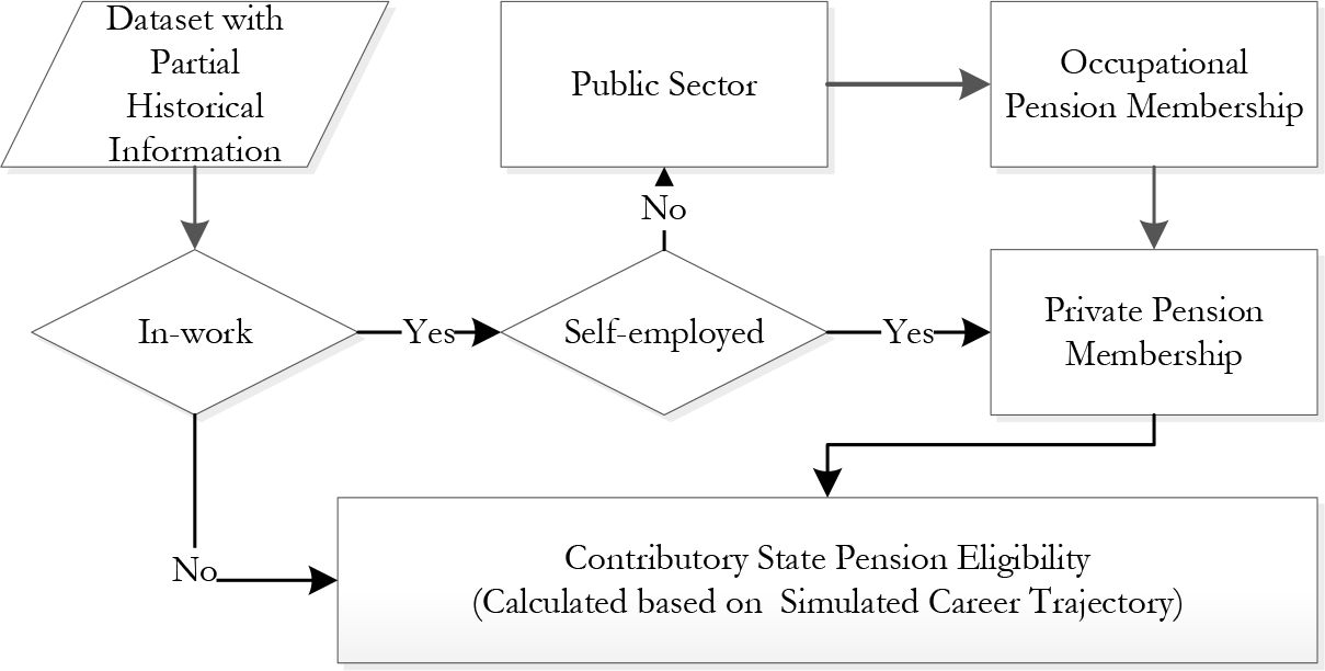
Simulation flowchart for the employment status variables.
The simulations are based on the complete sample of the 1994 population in the LII survey. Since the model does not generate historical profiles for people who have died before 1994, the simulated sample is not representative of the population prior to 1994. This implies that the average age in the earlier years of the simulation is significantly lower than the average age in the sample. Therefore, outputs are presented mostly by age group or cohort group in order to avoid misunderstandings.
As discussed in the earlier section, the main goal of the back simulation model is to recreate a sensible history for all individuals in the dataset. Therefore, it is essential that the model output can replicate what actually happened. In an ideal world, the model output should be compared with the actual data to see how well the model performs. However, the lack of real historical data is the very reason that the back simulation is required. In addition, it is not feasible to compare the model with other back simulation approaches, e.g. statistical matching method, in this particular case, as synthetic history recreation is the only option due to the data limitation. Therefore, the results of the model are mainly compared with the known benchmarks: the census reports and the pension eligibilities. A success replication of this information would suggest the simulated historical profiles are sensible at both aggregate and individual level.
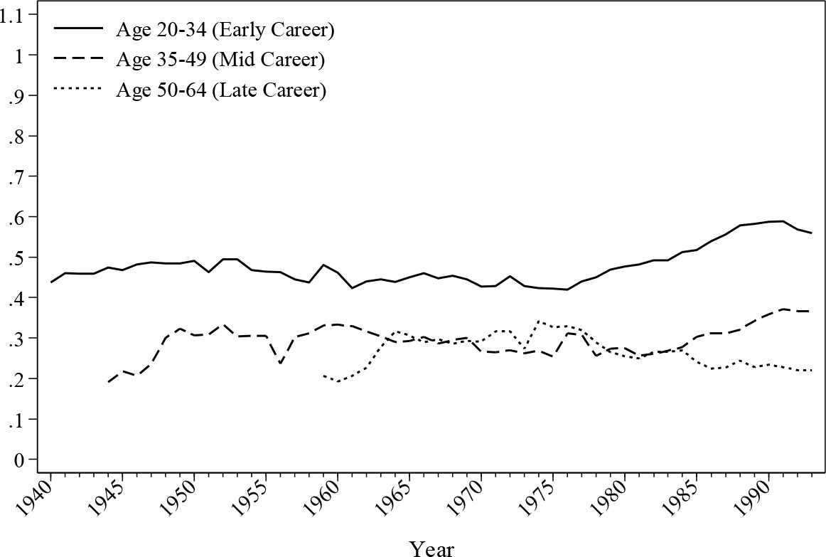
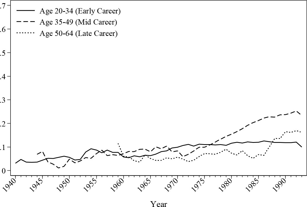
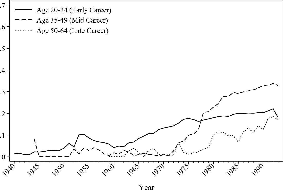
6.1 In-work ratio
The evolution of the in-work ratio is reproduced in Figure 2 and Figure 3. As the graphs show, the male employment rate alters little over time except for a gradual fall of late career employment since the introduction of the retirement pension system in the 1970s. The female employment rate is 40%~50% lower than the male employment rate throughout the simulated history. The simulation indicates that the female labour participation rate is much higher before the age of 35 than for other age groups.

Simulated historical in-work ratio for male by age.

Simulated historical in-work ratio for female by age.
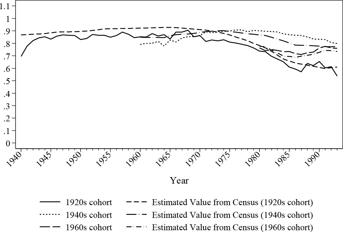
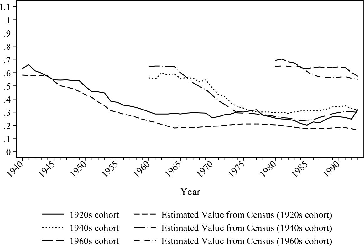
Figure 4 and Figure 5 further examine the simulated historical in-work proportion and offer a comparison with the census values to validate the simulation. As discussed earlier, the crosssectionals in the simulated period are not population representative due to the missing values of deceased individuals. Therefore, census values were adjusted based on the sample’s demographic features. In order to isolate the change of demographic composition, graphs are presented by cohorts.

Simulated historical in-work ratio for male by cohorts.

Simulated historical in-work ratio for female by cohorts.
The figures confirm that the simulated values roughly match the estimations from the census data with a deviation of around 5 percentage points on average. The simulation seems to work better for later cohorts than the earlier ones, however this difference may partially be caused by the longitudinal alignment procedure where the adjustments may not be perfectly balanced, and the inconsistencies in retrospective variables, where the data quality declines as age increases. Nonetheless, it is safe to say that the simulated ratios move in the same direction as the census values.
The back simulation module not only aims at providing a reasonable profile at the crosssectional level, but also a historical trajectory that is consistent with retrospective variables. Figure 6 illustrates the difference between the simulated number of years in work and the reported values. As shown, the longitudinal inconsistency in the simulation is well controlled; in total, over 83% of the individuals were simulated with an error no greater than 1 year, and over 89% of the observations have a difference of less than 2 years. A few extreme cases are also spotted with an error greater than 10 years. These observations typically report no working history but with old age pension entitlement. In this case, the model overrides the report of zero working year in favour of the observed pension eligibilities. On average, the absolute simulation errors for males are slightly larger than those for females. A possible reason is that males generally have longer career trajectories, which increase the computation complexity in balancing the crosssectional and longitudinal alignments. The longer career trajectory also implies that the measurement error of the retrospective values like reported years of work might be bigger for males. As a result, the quality of the simulation could be negatively affected due to the inconsistent reported values.

Difference between simulated years of work and reported value.
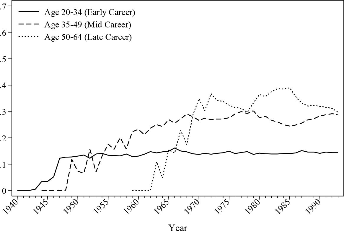
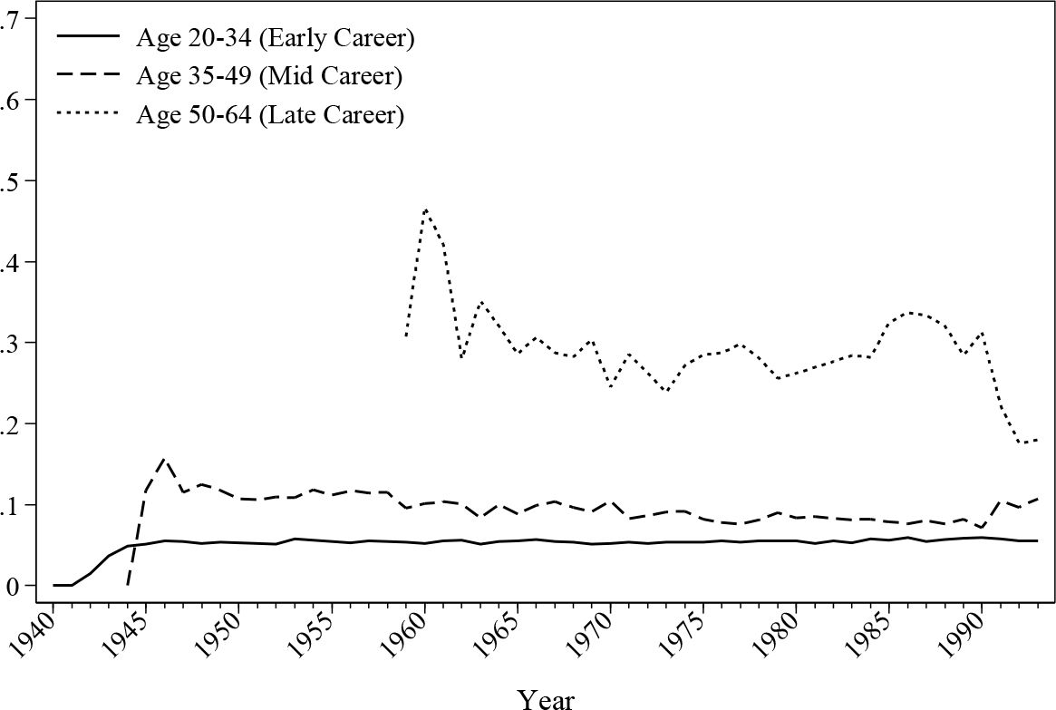
6.2 Employment sectors and self-employment
Figure 7 and Figure 8 depict the historical evolution of public sector employment by age. As shown, there is a gradual growth of public sector workers for all age groups, a trend that is consistent for both males and females. However, the increase of females working in the public sector is faster compared with male workers, especially for workers in their early and midcareer stages.

Public sector employment for male.
Simulated public sector employment for female.
Regarding the self-employed, Figure 9 and Figure 10 reveal the different preferences amongst different age groups. From the graphs it can be seen that the self-employment rates increase dramatically for males above the age of 35 over time and this stabilises around 30%, while the self-employment rate for males under 35 is just above 12% most of the time. The raise slope of the curve in the earlier part of the history may be contributed to by the limited number of observations for the age group. For females, the self-employment ratio is more or less stable within each age group except for a moderate decline for workers over 50 years old. Despite the drop, this late-career age group has a self-employment rate of around 30%, which is more than 20 percentage points higher compared with other groups. The differences are mainly due to the dropped female labour participation at later ages. Since the average age of retirement for female employee is lower than the male counterparts, the proportion of the self-employed workers increases after age 50. The graphs demonstrate that workers under the age of 35 have the least preference towards self-employment, a preference which is observed in both the simulated histories and the original dataset.

Simulated male self-employed ratio by age.

Simulated female self-employed ratio by age.
7. Results II: pension memberships and eligibilities
According to Irish pension regulations, individuals retiring at the age of 65 or later are entitled to a retirement or old age social welfare pension (RP and OAP, respectively), which can either be contributory or means-tested. The state pension system consists of a social insurance pension introduced for those aged 70+ in 1961 and a retirement pension for those aged 65 introduced in 1970 (O’Donoghue, 2002). Individuals may be entitled to additional pensions depending on their jobs and personal choices. The back simulation module replicates the pension system by simulating each individual’s participation in pension schemes and calculating their eligibility for a state pension once an individual retires.
7.1 State pension eligibilities
State pension eligibility is calculated from the simulated contribution history, which means that an output consistent with observed pension eligibility requires the complete working trajectory (employment status/type/sector) to be within a plausible and restricted range. Therefore, the consistency of pension eligibilities could be seen as an important indicator of overall simulation quality.
Table 7 lists the accuracies of different simulated pension eligibilities. Overall, the back simulation module developed in this paper is able to simulate the eligibility with an error of less than 5% for any pension type. This result is obtained after the longitudinal alignment procedure, which improved the accuracy of simulated eligibility by more than 25 percentage points in the exercise1.
Percentage of correctly simulated eligibility.
| Pension Type | Correctly Simulated | Number of Observations* |
| Contributory State Pension | 96.08% | 9,343 |
| Occupational Pension | 98.25% | 10,030 |
| Private Pension | 97.36% | 1,706 (Year 2000 onwards) |
-
*
Only those aged 66+ are included for state pension and those aged 65+ for occupational and private pension.
7.2 Occupational pension membership
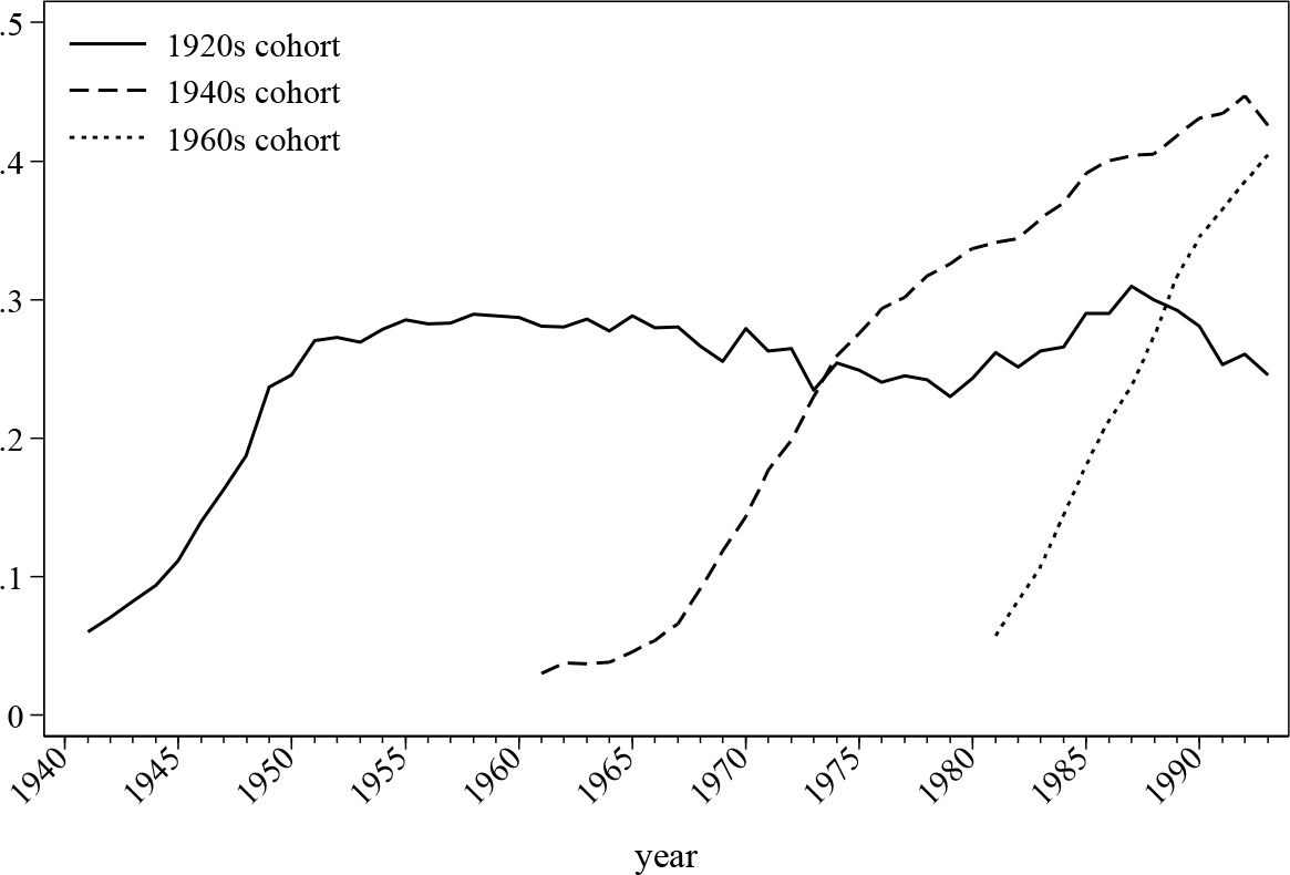
Occupational and private pensions are simulated through well-specified logit models and the results are aligned with the information extracted from the QNHS and LII survey2. Figure 11 describes the development of occupational pension membership by cohorts. It seems that later cohorts are more willing to participate in occupational pension schemes, which might imply an increase in the occupational pension coverage in Ireland over time, which in turn is consistent with the history of Irish pension reforms.

Occupational pension participation by cohort.
Analysing the trend for the cohort prospectively shows the dynamics of pension participation across time for the different cohort groups. Nonetheless, it does not reveal the dynamics of age preference, which is tightly linked with career development. Figure 12 discloses the shift of preference of same age groups across time. As suggested, mid-career individuals appear to be participating more actively then those in other groups. It seems that the age group closest to retirement has the lowest participation rate, which could due to the differences in career trajectories, availability of the pension options for this cohort and other reasons.
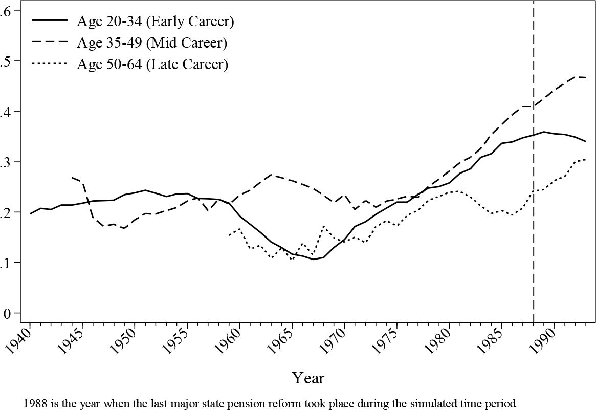
Occupational pension participation by age group.
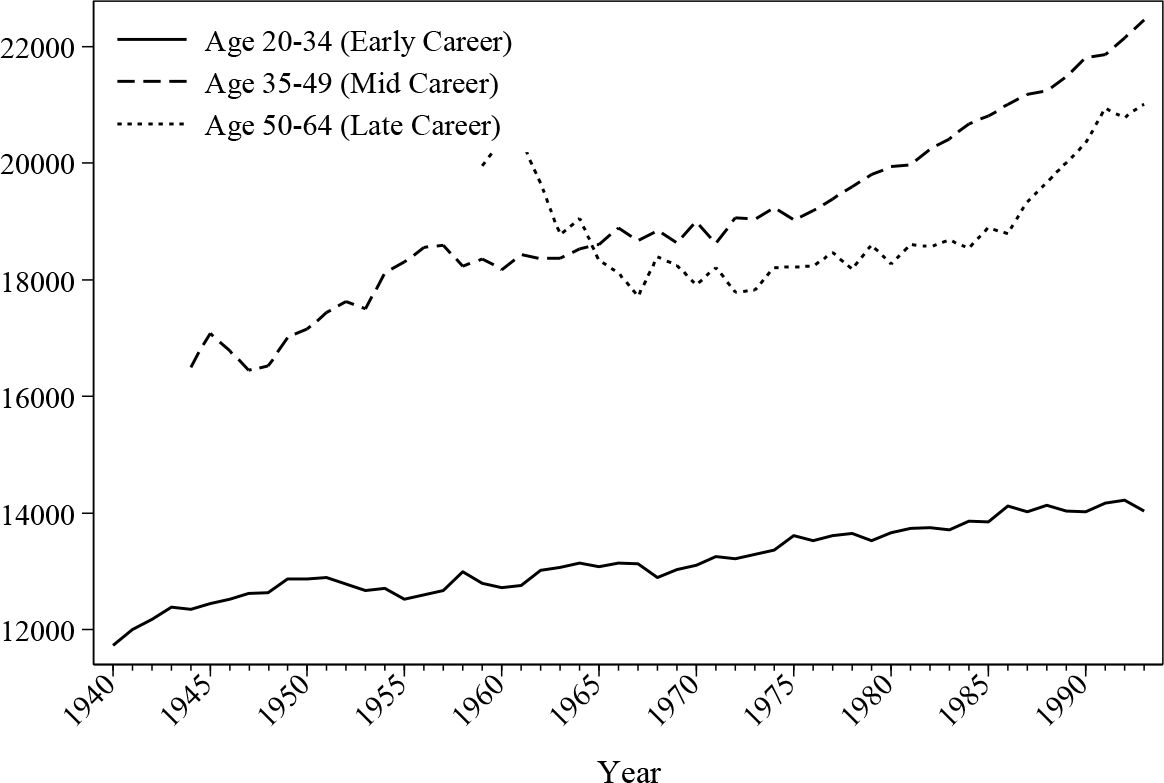
8. Results III: income variables
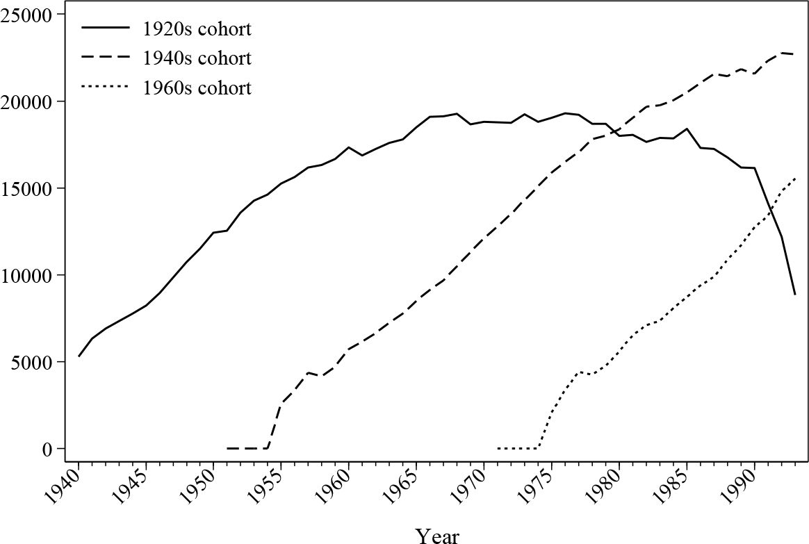
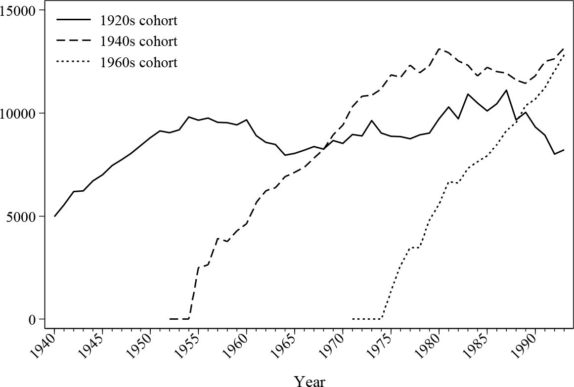
In addition to employment statuses, the back simulation module also provides monetary income histories for all individuals. Labour earnings are simulated using the models mentioned in Section 4, while other non-labour income is assumed stable over time as they do not affect pension memberships. Figure 13 and Figure 14 demonstrate the dynamics of the average labour income over lifetime in this back simulation by analysing the earnings of three different cohorts. The average earning curve, as shown by the earlier cohorts, has the distinctive shape of a quadratic function, which matches the expectation of classic human capital theory. Female earnings seem to have a more flat mid-career profile, which may be due to the career interruption caused by maternity leave.

Average male earnings (£) by cohort.

Average female earnings (£) by cohort.
Figure 15 and Figure 16 give an overview of the evolution of earnings across the different age groups. As can be seen, average earnings increase steadily due to the increasing level of education. This is also confirmed by the cohort graphs shown earlier, where the younger cohorts demonstrate higher peak values. Male earnings are substantially different depending on the stage of their career. The average earnings by age 50 or above can be more than 50% higher compared to a male aged 20–35, but the difference is a lot smaller for female workers.

Average male earnings (£) by age.

Average female earnings (£) by age.
9. Conclusions
As discussed above, the preparation of the base dataset is one of the most important elements in every dynamic microsimulation model. However, finding a long historical panel dataset with all the necessary variables is often infeasible. This paper develops an algorithm to simulate a historical panel for the LII dataset to fill in the missing history.
The back simulation module extracts retrospective information from the LII survey and applies a dynamic microsimulation in a reversed direction to simulate population histories. Due to the nature of historical simulation, the longitudinal consistency requirement is high and difficult to achieve when compared with a forward dynamic microsimulation. The method proposed in this paper solves this problem by introducing extra calibrations and alignments at both the crosssectional and longitudinal levels. The overall result of the simulated panel, as described in the earlier sections, matches the labour market history to a fairly high degree based on the macro statistics calculated. The simulated values follow the observed trend quite closely, and are able to pick up the dynamics of different types of pension eligibility across time and cohorts. Nevertheless, further validation of the long-term trajectories of the employment and earnings produced by the model might be necessary, although there is little reliable data to compare the results with for the earlier half of 20th century.
The back simulation method could potentially offer many benefits for microsimulation modellers. By expanding the longitudinal information while maintaining consistencies with a panel dataset with limited waves, it offers a viable alternative to the dilemma of base dataset choice as described by Cassells et al. (2006) and Zaidi and Scott (2001). The generated historical panel could consequently enhance the accuracy and stability of the forward dynamic simulation by feeding in information on career trajectory. Given the extensive retrospective information modelled, the back simulated panel has a much higher data quality than a simple synthetic panel. Since only standardized survey questions and macro statistics are used in the simulation, this proposed back simulation method could be potentially replicated in other datasets that include retrospective questions, e.g. ECHP, BHPS, German Socio-Economic Panel (GSOEP), FFS. The method could help modellers to run a life-cycle based simulation without using a scarce long panel. In addition, the historical panel provides many important insights, e.g. the dynamics of career trajectories, which would otherwise be easily overlooked in the original dataset.
The exploration of a back simulation method as described in this paper is still in its early stages and the current algorithm could be further improved. Future work is planned to improve the following aspects of the back simulation model:
Simulation of the deceased cohort of the population in order to align historical statistics more accurately, as the current version does not generate a representative historical population.
Develop an improved algorithm for the cross-sectional/longitudinal alignment to alleviate the impact of inaccurate responses for retrospective questions.
Understand the robustness of the model and the standard errors of the results. Further analysing the variations in the model would enhance the credibility of the model, especially when stochastic components are used.
In spite of the shortcomings inherent in the current version of this model, this paper shows that reconstructing historical information is feasible based on standard household survey dataset and census information, providing there is some retrospective information in the dataset that can be used for modelling. From a practical point of view, the simulated panel is the only available historical panel dataset for Ireland, which offers the possibilities of investigating life-cycle income profiles together with a dynamic microsimulation model.
Footnotes
1.
The effectiveness of the longitudinal alignment is determined by a number of factors, which include the number of iterations used, the balancing parameters between the cross-sectional accuracy and the longitudinal consistency, models used in the back simulation, and stochastic terms. The number illustrated here only reflects the efficiency of one particular run that produces the back simulation results in this paper.
2.
Using contemporary data for alignment might lead to overestimated pension participations. A better solution would involve gathering historical data and using it together with pension income, which could then potentially reveal the length of contributions. However, such an improved alignment is not possible in the current model given the availability of data.
Appendix 1 Steps of Back Simulation
Estimate models
Employment (in-work/out-of-work) model
Self-employed model
Impute social economic status variables for each year in the original dataset (1994-2001)
Impute the number of years in education, employment, sickness, home care duties and retirement using regression in 1994 by sex group
Update these variables to 1995–2001
Consistency check for major social economic variables during the years 1994–2001
Generate historical data using known information
Demographic information (e.g. year of birth)
Maternity information (based on child age)
Job information (e.g. year of starting first job, last job, total number of years worked etc.)
Pension information (e.g. total pension contribution, pension entitlements)
Others (e.g. school, geographic information)
Deterministic back simulation (in/out work)
Create age information
b. Infer working status from retrospective variables
Must be out of work before year of starting work
Must be in work in the year of starting work
Must be in work since the current job started
Must be in work in the year of quitting previous job
Must be unemployed since current unemployment started
Semi-stochastic back simulation
Assuming a 75% chance that a woman will be “out of work” in the year of giving birth to a child
State pensioners must start work before the age of 56
“Back to work” beneficiaries must have been unemployed for 2 years
Fill the gap of unallocated working status for history using stochastic simulation
Replace the unknown working status to “in work” if the number of known working years is lower than the total work years
Error term is stochastic. The ranking is based on the sum of the error terms and the personal effect in the model
The status is aligned with census data by interacting with the ranking
Impute the working status if there is still a gap between the reported number of years in work and the simulated years of in work
Set the rest of the employment statuses to “not in work” if the simulated number of years in work is consistent with the reported values
Adjust any differences
Simulate/Generate the variables that LIAM will use
Demographic information (age, alive, maternity)
Education information (based on the age of leaving full time education)
Marriage information
Calculate the year in which an individual married
Assume that an individual married at age 25 if the current marital status is separated, divorced or widowed.
d. Prepare employment information
Self-employment
Estimate the probability of being self-employed (1994–2001)
Read the historical values of self-employment and smooth the curve using moving average method
Use the stochastic term and personal effect to predict the probability of selfemployment, align data with estimates.
Public sector
Assume that people stick with the same sector as reported in 1994
Do not allow for small gaps in public sector employment
Store alignment data by sex education and cohort
Use stochastic term and personal effect to predict the probability of staying within the public sector, and align the data using saved values
Final adjustments to smooth labour participation history
Calculation for pay related social insurance (PRSI) pension entitlement
Create a variable for the contributory class in the PRSI system for state pensions
Public servants are treated as employees if they joined the job after 1995
Public servant pensions are eligible for those who joined the work before 1995
Calculate the eligibility for a PRSI pension for the rest
Self-employed are assumed to only be insured after 1988
Public sector are assumed to only be insured after 1995
Calculate the pension credit
Longitudinal Alignment
Compare simulated PRSI pension entitlement with the actual entitlement
Modify the history while keeping the cross-sectional alignment of the labour market participation, self-employed and pension coverage ratio stable
Repeat the above procedure several times until the consistency is satisfactory
Simulate earnings (for employees and self-employed)
Estimate the wage model (random effect model)
Record the standard deviation of random effects and the error term
Simulate the wage for each group with a stochastic term that shares the standard deviation of estimated random effects
Align the average earnings by sex, education level and age group to the year 2000 values
Simulate occupational pension membership using the equation estimated using the 1994-2001 data and calibrated using the QNHS samples.
Calculate the probability of receiving an occupational pension, employee personal pension and self-employed personal pension for each age and sex group
Estimate the occupational/self-employed/personal pension model using existing data
Align it with the probability breakdown calculated from the QHNS sample for both the existing dataset (LII) values and the simulated historical values
Correction for the unlikely event of an inconsistency between the occupational pension status and the employment status
Final adjustment and alignment
Calculate the value of the DC Occupational pension fund
Model contribution in a similar manner as wages and align with observed contribution rate (split into two rates, pre-1995 and post-1995)
Calculate the pension fund value from the 1930s using assumed interest rates
Calculate the contributions for each pension type
Appendix 2 Estimates for Certain Retrospective Variables (Male)
| Variables | Equations | |||
|---|---|---|---|---|
| Years in full-time education or training | Years in employment, self-employment or farming | |||
| coefficient | s.e. | coefficient | s.e. | |
| College Education | 4.22 | 0.07 | −3.43 | 0.21 |
| Secondary Education | 2.17 | 0.07 | −1.66 | 0.21 |
| Age | 0.00 | 0.02 | 0.36 | 0.05 |
| Is Working | −1.02 | 0.13 | 7.37 | 0.37 |
| Illness | 0.16 | 0.14 | −1.99 | 0.42 |
| In education | −0.89 | 0.14 | 2.85 | 0.41 |
| Unemployed | −1.28 | 0.14 | 1.03 | 0.40 |
| Retired | −1.05 | 0.17 | 4.30 | 0.51 |
| Number of Children under Age 3 | −0.06 | 0.06 | 0.16 | 0.19 |
| Number of Children between Age 4 and 11 | −0.10 | 0.03 | 0.09 | 0.10 |
| Number of Children between Age 12 and 15 | −0.09 | 0.04 | 0.06 | 0.12 |
| Cohort Dummies | Yes | Yes | Yes | Yes |
| Number of Observations | 5,738 | 5,738 | ||
| Adjusted R-square | 0.48 | 0.90 | ||
| Variables | Equations | |||
|---|---|---|---|---|
| Years in unemployment | Years of illness/disabled | |||
| coefficient | s.e. | coefficient | s.e. | |
| College Education | −1.05 | 0.11 | −0.02 | 0.10 |
| Secondary Education | −0.79 | 0.11 | −0.03 | 0.10 |
| Age | −0.01 | 0.02 | 0.05 | 0.02 |
| Is Working | −0.04 | 0.19 | −0.80 | 0.18 |
| Illness | −1.33 | 0.21 | 3.78 | 0.20 |
| In education | 0.61 | 0.21 | −0.23 | 0.20 |
| Unemployed | 3.91 | 0.21 | 1.17 | 0.19 |
| Retired | 1.01 | 0.26 | −1.46 | 0.24 |
| Number of Children under Age 3 | −0.03 | 0.10 | 0.07 | 0.09 |
| Number of Children between Age 4 and 11 | 0.06 | 0.05 | −0.04 | 0.05 |
| Number of Children between Age 12 and 15 | 0.10 | 0.06 | −0.13 | 0.06 |
| Cohort Dummies | Yes | Yes | Yes | Yes |
| Number of Observations | 5,738 | 5,738 | ||
| Adjusted R-square | 0.23 | 0.15 | ||
| Variables | Equations | |||
|---|---|---|---|---|
| Years spent on home duties | Years in retirement | |||
| coefficient | s.e. | coefficient | s.e. | |
| College Education | 0.43 | 0.12 | 0.00 | 0.07 |
| Secondary Education | 0.40 | 0.12 | −0.01 | 0.07 |
| Age | −0.12 | 0.03 | 0.03 | 0.02 |
| Is Working | −2.35 | 0.21 | −0.25 | 0.12 |
| Illness | 0.62 | 0.24 | −0.05 | 0.13 |
| In education | −2.20 | 0.24 | −0.22 | 0.13 |
| Unemployed | −2.28 | 0.23 | −0.20 | 0.13 |
| Retired | −2.42 | 0.29 | 5.65 | 0.16 |
| Number of Children under Age 3 | 0.20 | 0.11 | −0.01 | 0.06 |
| Number of Children between Age 4 and 11 | −0.06 | 0.06 | −0.03 | 0.03 |
| Number of Children between Age 12 and 15 | 0.04 | 0.07 | −0.02 | 0.04 |
| Cohort Dummies | Yes | Yes | Yes | Yes |
| Number of Observations | 5,738 | 5,738 | ||
| Adjusted R-square | 0.03 | 0.74 | ||
Appendix 3 Estimates for Certain Retrospective Variables (Female)
| Variables | Equations | |||
|---|---|---|---|---|
| Years in full-time education or training | Years in employment, self-employment or farming | |||
| coefficient | s.e. | coefficient | s.e. | |
| College Education | 3.47 | 0.07 | −0.54 | 0.29 |
| Secondary Education | 2.01 | 0.06 | −0.06 | 0.26 |
| Age | 0.02 | 0.01 | 0.05 | 0.06 |
| Is Working | 0.34 | 0.06 | 8.34 | 0.28 |
| Illness | −0.32 | 0.12 | 0.06 | 0.53 |
| In education | 0.21 | 0.11 | 2.79 | 0.48 |
| Unemployed | 0.96 | 0.13 | 4.00 | 0.55 |
| Retired | 0.53 | 0.13 | 26.78 | 0.59 |
| Number of Children under Age 3 | −0.07 | 0.05 | 1.26 | 0.23 |
| Number of Children between Age 4 and 11 | −0.03 | 0.03 | 0.27 | 0.13 |
| Number of Children between Age 12 and 15 | −0.06 | 0.04 | −0.75 | 0.16 |
| Cohort Dummies | Yes | Yes | Yes | Yes |
| Number of Observations | 5,725 | 5,725 | ||
| Adjusted R-square | 0.50 | 0.54 | ||
| Variables | Equations | |||
|---|---|---|---|---|
| Years in unemployment | Years of illness/disabled | |||
| coefficient | s.e. | coefficient | s.e. | |
| College Education | −0.37 | 0.06 | −0.25 | 0.09 |
| Secondary Education | −0.30 | 0.05 | −0.26 | 0.08 |
| Age | 0.01 | 0.01 | −0.03 | 0.02 |
| Is Working | 0.18 | 0.06 | −0.26 | 0.09 |
| Illness | −0.20 | 0.11 | 2.55 | 0.17 |
| In education | 0.16 | 0.10 | −0.10 | 0.15 |
| Unemployed | 1.74 | 0.12 | 0.30 | 0.17 |
| Retired | 0.65 | 0.12 | 0.27 | 0.19 |
| Number of Children under Age 3 | 0.03 | 0.05 | −0.02 | 0.07 |
| Number of Children between Age 4 and 11 | −0.03 | 0.03 | −0.11 | 0.04 |
| Number of Children between Age 12 and 15 | 0.00 | 0.03 | −0.24 | 0.05 |
| Cohort Dummies | Yes | Yes | Yes | Yes |
| Number of Observations | 5,725 | 5,725 | ||
| Adjusted R-square | 0.06 | 0.05 | ||
| Variables | Equations | |||
|---|---|---|---|---|
| Years spent on home duties | Years in retirement | |||
| coefficient | s.e. | coefficient | s.e. | |
| College Education | −1.87 | 0.34 | −0.10 | 0.07 |
| Secondary Education | −1.03 | 0.30 | −0.04 | 0.06 |
| Age | 0.22 | 0.07 | 0.03 | 0.02 |
| Is Working | −8.58 | 0.32 | 0.01 | 0.07 |
| Illness | −1.65 | 0.62 | 0.05 | 0.13 |
| In education | −5.04 | 0.56 | −0.01 | 0.12 |
| Unemployed | −7.31 | 0.64 | −0.02 | 0.13 |
| Retired | −34.35 | 0.69 | 8.96 | 0.14 |
| Number of Children under Age 3 | −0.66 | 0.27 | −0.03 | 0.06 |
| Number of Children between Age 4 and 11 | −0.03 | 0.15 | 0.03 | 0.03 |
| Number of Children between Age 12 and 15 | 0.42 | 0.18 | −0.05 | 0.04 |
| Cohort Dummies | Yes | Yes | Yes | Yes |
| Number of Observations | 5,725 | 5,725 | ||
| Adjusted R-square | 0.75 | 0.46 | ||
Appendix 4 Estimates for Earnings
| Male Employee Earnings | Female Employee Earnings | Self-employment Earnings | |
|---|---|---|---|
| College Education | 0.56 | 0.81 | 0.72 |
| (0.03) | (0.03) | (0.06) | |
| Secondary Education | 0.31 | 0.49 | 0.31 |
| (0.03) | (0.03) | (0.06) | |
| Work Experience (Years) | 0.09 | 0.05 | 0.03 |
| (0.00) | (0.00) | (0.00) | |
| Work Experience (Squared) | 0.00 | 0.00 | 0.00 |
| (0.00) | (0.00) | (0.00) | |
| Years of Unemployment) | 0.04 | 0.01 | 0.01 |
| (0.00) | (0.00) | (0.00) | |
| Gender (Male=1) | 0.44 | ||
| (0.06) | |||
| Total Number of Observation | 13678 | 10231 | 5092 |
-
(standard errors are reported in the parenthesis).
References
-
1
Un outil de prospective des retraites: le modèle de microsimulation DestinieÉconomie et prévision pp. 193–214.
- 2
-
3
Problems and Prospects for Dynamic Microsimulation: A Review and lessons for APPSIM. NATSEM Discussion PaperProblems and Prospects for Dynamic Microsimulation: A Review and lessons for APPSIM. NATSEM Discussion Paper.
- 4
-
5
Individual alignment and group processing: an application to migration processes in DYNACAN, occasional papers-university of Cambridge department of applied economics238–250, Individual alignment and group processing: an application to migration processes in DYNACAN, occasional papers-university of Cambridge department of applied economics.
-
6
PENSIM: A Dynamic Simulation Model of Pensioners’ Income ” in Government Economic Service Working Paper No. 129London: Analytical Services Division, Department of Social Security.
-
7
Microsimulation Modelling for Policy Analysis: Challenges and InnovationsSimulating Transitions Using Discrete Choice Models, Microsimulation Modelling for Policy Analysis: Challenges and Innovations, Cambridge, Cambridge University Press.
- 8
-
9
Imputing pension and caring histories to the base data in the SAGE dynamic microsimulation modelSAGE Technical Note No 8.
-
10
A Primer on the Dynamic Simulation of Income Model (DYNASIM3)A Primer on the Dynamic Simulation of Income Model (DYNASIM3).
-
11
Using The Eu Silc For Policy Simulation: Prospects. Some Limitations And Suggestions, EUROMOD Working PapersUsing The Eu Silc For Policy Simulation: Prospects. Some Limitations And Suggestions, EUROMOD Working Papers.
-
12
Can we Afford the Future? An evaluation of the new Swedish pension system, Modelling our future: population ageingsocial security and taxation 33.
-
13
The MOSART model-a short technical documentationThe MOSART model-a short technical documentation.
-
14
Challenges and Opportunities of Dynamic Microsimulation ModellingChallenges and Opportunities of Dynamic Microsimulation Modelling.
- 15
-
16
Pension incomes in the European Union: policy reform strategies in comparative perspectiveMicro-simulation in action: policy analysis in Europe using EUROMOD 27.
-
17
Labor mobility and wages, Studies in Labor Markets2164, Labor mobility and wages, Studies in Labor Markets.
-
18
DYNACAN, the Canadian pension plan policy model: demographic and earnings componentsProceedings of the Microsimulation Section at the International Conference on Information Theory, Combinatorics, and Statistics.
-
19
Overview of DYNACAN, a full-fledged Canadian actuarial stochastic model designed for the fiscal and policy analysis of social security schemesOverview of DYNACAN, a full-fledged Canadian actuarial stochastic model designed for the fiscal and policy analysis of social security schemes.
- 20
-
21
Dynamic microsimulation: a methodological surveyBrazilian Electronic Journal of Economics 4:77.
- 22
-
23
The Life-Cycle Income Analysis Model (LIAM): A Study of a Flexible Dynamic Microsimulation Modelling Computing FrameworkInternational Journal of Microsimulation, 2, 1.
- 24
-
25
Estimation of earnings in the SAGE dynamic microsimulation model: London. ESRC-Sage Technical NoteEstimation of earnings in the SAGE dynamic microsimulation model: London. ESRC-Sage Technical Note.
-
26
Base dataset for the SAGE model. Sage Technical NoteBase dataset for the SAGE model. Sage Technical Note.
Article and author information
Author details
Acknowledgements
The authors are grateful to the National Research Fund, Luxembourg for the financial support. For their helpful discussions and comments, the authors wish to thank Elisa Baroni, Gijs Dekkers, two anonymous referees, and the participants of the 2010 European workshop on dynamic microsimulation modelling in Brussels.Text of acknowledgement
Publication history
- Version of Record published: June 30, 2012 (version 1)
Copyright
© 2012, Li & O’Donoghue
This article is distributed under the terms of the Creative Commons Attribution License, which permits unrestricted use and redistribution provided that the original author and source are credited.