Linking a microsimulation model to a dynamic CGE model: Climate change mitigation policies and income distribution in Australia
- Melbourne Institute of Applied Economic and Social Research, Australia
- Article
- Figures and data
- Jump to
Abstract
This paper extends the ‘top-down’ framework developed by Robilliard et al. (2001) to link a computable general equilibrium (CGE) model to a microsimulation (MS) model. The proposed approach allows for the linking of an MS model to a dynamic (rather than static) CGE model. The approach relies on altering the sample weights in order to reproduce long-term population projections and changes in employment as estimated by the CGE model. The approach is applied to assess the effects of climate-change mitigation policies in Australia from 2005 to 2030 at five-yearly intervals.
1. Introduction
This paper outlines an approach to disaggregate the results of a dynamic economy-wide computable general equilibrium (CGE) model into results at the household and individual level by using a microsimulation (MS) model. In this analysis, the CGE results had to be taken as given, and it is the MS model that is adapted to use all relevant inputs from the CGE model.
The proposed approach is applied to predict the effects of climate-change mitigation policies on income and inequality in Australia for the period from 2005 to 2030. The modelling of the economy-wide effects of climate-change mitigation policies is a fast-growing field, and this paper makes use of the first such study in Australia. However, how these economy-wide effects impact household income distribution remains a less-researched question. The aim of this paper is to provide both a valid methodological approach to answer this question and a first application.
Three scenarios are considered in the simulations. The only difference between the two mitigation scenarios and the reference scenario is the introduction of an Emissions Trading Scheme on 1 July 2013. The Garnaut Climate Change Review (2008) lists in great detail how the mitigation scenarios are translated into shocks which form the input for the CGE. Only key areas of impact from climate change, for which the impacts could be measured with enough certainty to be modelled in the CGE, were included. Broadly speaking, it determined the likely market impacts of climate change on primary production (sheep and cattle, dairy, cereals), critical infrastructure (coastal settlements, water and electricity, transport), human health (heat stress, illnesses, and their effect on productivity and labour supply), and tropical cyclones (capital losses from storms). Most of these impacts were operationalised by changes in primary factor usage, capital augmenting technical change, intermediate input technical change, effective labour supply, and labour productivity. The two mitigation scenarios differ in the level with which emissions are to be reduced. It is assumed that climate change itself will not have a direct economic impact before 2030.
The proposed approach draws on the ‘top-down’ framework introduced by Robilliard et al. (2001) in which the CGE model is run in a first step and the changes are passed on to the MS model in a second step1. However, in order to transmit employment changes from the CGE to the MS model, a reweighting procedure is used instead of the behavioural component of an MS model. 2 This alternative approach is preferred in the dynamic framework because it is then relatively easy to incorporate the benchmarks required to reproduce the demographic changes predicted to occur in the base population over the relevant period of analysis.3
The focus of the paper is on the methodology developed to link a dynamic economy-wide CGE model, the Monash Multi-Regional Forecasting (MMRF)-Green model (see Adams et al., 2002, 2007), to an MS model, the Melbourne Institute Tax and Transfer Simulator (MITTS; see Creedy et al., 2002). The paper provides an overview of the relevant assumptions made in both models as well as in the linking process. In addition, it discusses the limitations of the modelling approach and the initial discrepancies between the two models. As an illustrative example, the approach is applied to assess the effects of climate-change mitigation policies in Australia from 2005 to 2030. The CGE model used in this paper was developed as part of the Garnaut Review on climate change (Commonwealth of Australia, 2008). The CGE results are used as exogenous inputs in our analysis. That is, the CGE results are a given in this paper and the aim is to make the best possible use of the MS model to produce estimated effects on income distribution. Therefore a brief description of MITTS is provided in Section 2 while the CGE model and assumptions are only discussed where relevant to MITTS.4 Where relevant, we do point out how an integrated approach of constructing a CGE and an MS model while keeping linking in mind during the design phase would have been able to provide a deeper understanding and finer breakdown of results taking into account greater levels of heterogeneity.
The structure of the paper is as follows. Following the description of MITTS in Section 2, a detailed discussion of the linking approach is given in Section 3. Section 4 presents the results on income for the reference case and the two mitigation scenarios. Section 5 concludes.
2. The melbourne institute tax and transfer simulator
MITTS is a behavioural MS model, but for this analysis only the non-behavioural component is used.5 The employment changes predicted by the CGE model, as well as the changes in the base population, are reproduced using a reweighting procedure in MITTS. Then MITTS computes net household incomes for a representative sample of households, for both incumbent and counterfactual tax-benefit regimes. A major advantage of MS modelling is that such modelling retains the full extent of the heterogeneity contained in the survey data used.
This subsection first describes the arithmetic MS model, followed by a discussion of the data required to build this type of model (see Creedy et al., 2002 for more details).
2.1 The arithmetic model
When examining the effects of policy changes, analyses generally rely on tabulations and associated graphs, for demographic groups, of the amounts of tax paid (and changes in tax) at various percentile income levels. The more sophisticated models may have extensive ‘back end’ facilities allowing computation of a range of distributional indicators (such as the Gini coefficient) and tax progressivity measures, along with social welfare function evaluations in terms of incomes. Arithmetic models are typically used to generate profiles, again for various household types, of net income at a range of gross income levels.
Since the first version of MITTS was completed in 2000, it has undergone a range of substantial developments and data updates. In the present version, the Survey of Income and Housing Costs (SIHC) data from 1994/1995, 1995/1996, 1996/1997, 1997/1998, 1999/2000, 2000/2001, 2002/2003, 2003/2004 and 2005/2006 can be used6. Results are aggregated to population levels using the household weights provided with the SIHC.
In MITTS, the arithmetic tax and benefit modelling component is called MITTS-A. The tax system component of MITTS contains the procedures for applying each type of tax and benefit. Each tax structure is associated with a data file containing the corresponding tax and benefit rates, benefit levels and income thresholds used in means testing. In view of some data limitations of the SIHC, it is not possible to include within MITTS all the complexity of the tax and transfer system. However, all major social security payments and income taxes are included7.
Pre-reform net incomes at the alternative hours levels are based on the MITTS calculation of entitlements, not the actual receipt. In the calculation of net income a 100 per cent take-up rate is assumed. This is likely to cause overestimation of government expenditure on some of the payments. However, it should have little impact on the results since both the amounts in the reference case and in the mitigation scenarios will be overestimated. Furthermore, in this paper it is assumed that benefit rates and benefit threshold incomes remain the same in real terms. However, alternative tax and transfer systems are still required in this analysis to account for the indexation of income tax thresholds to real wages.
The various components of the tax and benefit structure are assembled in the required way in order to work out the transformation between hours worked and net income for each individual under each tax system. For example, some benefits are taxable while others are not, so the order in which taxes and transfers are calculated is important.
2.2 The data
The distinguishing feature of MS models is the use of a large cross-sectional and nationally representative dataset with the characteristics of individuals and households, including their labour supply, earnings and (sometimes) expenditure. MS models are therefore able to replicate closely the considerable degree of heterogeneity observed in the population. The two large-scale household surveys that are potentially useful in the Australian context are the Household Expenditure Survey (HES) and the SIHC. The former does not contain sufficient information about hours worked by individuals while the latter does not contain information about expenditure patterns. The SIHC is a representative sample of the Australian population, containing detailed information on labour supply and income from different sources, in addition to a variety of background characteristics of individuals and households. The measurement of income in the HES is known to be unreliable, so that in developing models for the analysis of direct taxes and transfer payments reliance has been placed on the SIHC8.
When analysing actual or proposed policy changes, it is preferred to use data as close to the relevant time period as possible to avoid having a starting point that is too different from reality. When this is not possible, all monetary variables are uprated to the relevant year; that is, for example, in our analysis the amounts of income in 2003/2004 are increased to reflect January 2006 amounts or January 2010, 2015 etc. amounts. To uprate non-labour incomes, the Consumer Price Index (CPI) is used. To uprate wage rates, the average male and female wage indices are used for 2005, while the CGE model’s regional wage indices are used in subsequent years. Wage indices usually increase at a faster rate than the CPI.
3. Linking the MS to the CGE model: methodology
The variables used in making the link between the CGE model, MMRF, and the MS model, MITTS, are central to the analysis in this paper. All variables from the CGE model affecting the structure of the Australian population, household incomes or expenditures are relevant. Households derive most of their income from labour market activities, so any changes affecting wages or employment are particularly important. In addition to transferring this information for each point in time considered (that is, years 2010, 2015, 2020, 2025 and 2030) and for each policy run, the MS model needs to replicate the assumptions made by the CGE model about the evolution of the population and the labour force.
3.1 Population and employment changes: the reweighting approach
The Australian population is not explicitly modelled in the CGE model. Instead, changes in the population as predicted by Treasury (Commonwealth of Australia, 2008; Commonwealth Treasury, 2008) based on Australian Bureau of Statistics (ABS) data (2005, series B) are used to derive changes in the labour force, which in turn determine changes in labour supply. Treasury predicts the Australian population by age and gender up to 2050 starting from ABS (2005, series B) projections for the Australian population by age, gender and region up to 2050. However, the Treasury projections diverge from the ABS projections over time. Treasury’s projections form the base of the underlying population projections in the CGE model. However, the ABS projections are used to derive regional populations, since Treasury projections are only available at the national level. This combined approach allows us to follow CGE assumptions as closely as possible.
We use State population sizes as predicted by the CGE model. State populations are the same across the reference case and the two scenarios, but vary over time through interstate migration and population growth. Immigration flows, which are quite substantial in Australia, are accounted for by population growth projections as well.
The CGE model also estimates changes in employment levels by industry and region in a general equilibrium framework. The assumption in the CGE modelling is that employment levels by industry and region are determined by the model (that is, they are endogenous to the model) and the long-run rate of unemployment is assumed to be fixed. Since the industry classification is more aggregated in the MS model than in the CGE model, the changes in employment by industry provided by the CGE model are combined into 13 industry groups which are identifiable in the MS model9. In addition, the CGE model provides the number of unemployed persons by region.
The base file used in the MS analysis is the ABS 2003/2004 SIHC, which has been uprated to the financial year 2005/2006 within the MS model. The MS model needs to be benchmarked based on the information from the CGE model so that the initial population and labour force in the starting year in the MS model are consistent with the CGE model. In addition to reweighting these data for the base year, the base file used in the MS model needs to be reweighted separately for every year for which a simulation is run, benchmarking the MS model input data against the CGE model output to reproduce the required employment and population changes over time. A reweighting approach is used to map the base levels and changes as predicted by the CGE model to the MS model environment. This approach relies on adjusting the household weights in the SIHC so that changes in the relative and absolute size of various subgroups of the population are accounted for.
Consistency between the MS and CGE model is ensured in two reweighting steps as explained below. The structure of the population by age, gender and region provided by Treasury+ABS projections is altered by the interstate migration as predicted by the CGE model. This results in a different regional composition of the population by age and gender. Ideally, the MS model should be benchmarked to the CGE model but the information available from the CGE model is too aggregated to provide the MS model with a sufficiently detailed description of the Australian population. Therefore we need to use two separate projections. The approach has to be broken down into two steps, because the MS model cannot be benchmarked to both projections at the same time since they are not entirely consistent with each other. In addition, it should be noted that even if the CGE model were fully consistent with Treasury+ABS projections, two steps would still be required since we need to benchmark the MS model against a large number of constraints. Given that there are limitations on the number of constraints that can be used in calibrating the new weights, two steps are also needed to accommodate all required benchmarks. The first step ensures consistency with Treasury+ABS population projections. Then, a second reweighting step ensures consistency with the CGE model’s employment and unemployment projections, and updated interstate migration estimates.
In the first step, the underlying CGE population projections are imposed on the MS model using Treasury population projections, supplemented by the ABS regional decomposition (2005, series B). This is achieved by reweighting our basic sample from 2003/2004 to reflect updated benchmarks in terms of age and gender by region as predicted by Treasury+ABS.
The base file of the MS model is reweighted following the approach by Deville and Sarndal (1992) and Cai et al. (2006). In order to calculate the new weights, benchmarks from the Treasury and ABS are used; these include the population size and composition by age, gender and region. The reweighting approach aims to achieve specified population totals for selected variables, subject to the constraint that the adjustments to the original weights are as small as possible. Technical details are provided in Appendix 1.
In the second step, the same reweighting approach is applied to account for changes in employment levels by industry and region, unemployment levels by region, and interstate migrations as estimated by the CGE model. Employment levels in the MS model are benchmarked against employment levels by industry and region in the CGE model. As explained above, the CGE model industries are grouped so that they can be mapped to the 13 industries distinguished in the MS model. The reweighting process is subject to a number of constraints (representing the various benchmarks with regard to employment, unemployment and State populations) which ensure that the MS model reproduces the changes predicted by the CGE model in terms of interstate migrations, and employment and unemployment levels by region.
However, imposing all these constraints while not controlling for continued consistency with the Treasury projections could result in substantial discrepancies. For example, reweighting with regard to unemployment levels could affect the structure of the total population by age and gender since the unemployed are likely to have different characteristics compared to the rest of the population. To avoid such discrepancies, benchmarks for age and gender composition at the national level are also imposed at the second stage of the reweighting. Although these constraints ensure that the MS model remains consistent with the Treasury population projections by age and gender at the national level, in practice, discrepancies can still occur at the regional level. This is the case essentially because Treasury+ABS projections are altered by the CGE model, but the CGE model does not provide information about the new age and gender structure of regional populations. The two-step reweighting approach ensures that the MS model is consistent with the CGE model and that the deviations between the MS model and Treasury+ABS projections are minimised.
3.2 Labour and non-labour income
In the base year of 2005/2006, the CGE model accounts for wage differences by industry and region. In policy runs, the wage rates for different industries are presumed to move proportionally, that is, the pre-existing wage differentials between industries are held constant. Wage growth itself is largely determined by labour productivity growth, which is exogenous in the CGE model and based on Treasury and ABS projections (see Commonwealth Treasury, 2008). However, regional wage differentials are endogenously determined by the CGE model. Hence, the CGE model generates changes in average wages by region but not by industry (nor occupation). This has the disadvantage that there is no opportunity for skill levels to affect wage growth in the CGE model, and therefore current wage differentials between low- and high-skilled individuals are held constant in relative terms. Therefore, the information transferred to the MS model cannot account for changing wage differentials by skill level, which would otherwise have been likely to contribute to changes in income inequality. This limitation is due to the inherent lack of detail of such a large-scale modelling exercise. It also highlights how designing CGE and MS models with linking in mind could overcome this. Allowing for wage and employment changes by occupation or skill level in the CGE model, something highly desirable from the perspective of the MS model, would probably have come at the expense of richness in the CGE elsewhere. But it is only by developing both models simultaneously that the necessary trade-offs would result in the best possible outcome for the linked model.
The information on income in the MS model is very detailed. Information on all income components is available either at the household or individual level. In the MS model, labour income is determined at the individual level whereas the CGE model only estimates average changes in wages by region. The average changes estimated by the CGE model concern gross wages and these are used to uprate gross hourly wage rates in the MS model. Consequently, within each State, the current relative wage differential between two given workers is assumed to be fixed. However, changes in the wage distribution are generated by changes in employment levels by industry, since each industry has a different wage distribution. The wage distribution is also indirectly affected by the predicted changes in the population structure by age and gender, since wages vary among workers of different demographic groups. Hence, the CGE model changes are adjusted before being applied to each household in the MS model, so that the component of these changes due to changes in the population (and employment) structure is removed. This is necessary to avoid double counting since these structural changes are already accounted for by the reweighting10.
Similarly, information about non-labour income is only available at the regional level in the CGE model. The various non-labour income components are aggregated into two broad components: (i) non-labour factor income (mainly capital income), and (ii) individual benefit payments from the government with four subcategories: unemployment, disability, age and other. Following the CGE model assumptions, all individual benefit payments in the MS model are indexed to the CPI in order to be held constant in real terms.
The use of uprated gross wages and non-labour factor income, combined with observed labour supply for each individual, enables the calculation of income tax and social security payments using the tax and social security system of January 2006 (this is in the middle of the base financial year used in the CGE model). Since the CGE model only generates average changes by region, the average changes in the two non-labour income components corresponding to their region of residence are used for each household in the MS model. The four components of non-labour factor income available in the MS model, which include income from own unincorporated business, total income from investments, income from child support or maintenance, and other regular payments, are increased (or decreased) by the same percentage as predicted by the CGE model.
Since individual benefit payments from the government are fixed in real terms in the CGE model, the same assumption is made in the MS model.11 However, small changes in individual benefit payment levels may still occur at the individual level because eligibility to all individual benefit payments is determined endogenously by the MS model taking into account gross incomes. The MS model only uses gross income (both labour and non-labour income) from households as an exogenous input, from which it calculates income tax paid and income support received according to a set of taxation and social security rules. The rules usually vary by household composition (also exogenous to the model). using gross income combined with the computed amounts of income tax and income support payments, net income can be calculated.
Only income changes in real terms are used as input to the MS component so that other eligibility criteria do not have to be uprated to account for inflation. However, income tax thresholds are indexed to real wages in order to hold the national average tax rate more or less constant, in accordance with the CGE model assumptions (see Section 4.1 for more detail).12
Tax and transfer MS models are particularly strong on the calculation of net (or disposable) income starting from individuals’ gross incomes. As a result, establishing the link with the CGE model then allows for the calculation of individuals’ gross incomes —based on their wage, labour supply and other non-labour income—, total income tax and social security payments. Therefore, it is possible to calculate households’ disposable incomes under each of the policy runs. Real incomes adjusted for household-specific consumption patterns are computed for each scenario and the reference case, using price and consumption changes from the CGE model and the information from the Household Expenditure Survey (HES). Net incomes are expressed in 2005/2006 or base year prices. Table 1 describes the approach used in calculating household-specific CPIs. The cumulative price changes combined with the previous period’s budget shares are used. This approach accounts for changes in consumption patterns over time.13
Computation of household real income for one particular household.
| 2005 (base) | 2010 | 2015 | 2020 | 2025 | 2030 | |
|---|---|---|---|---|---|---|
| Nominal household income | y0 | y1 | y2 | y3 | y4 | y5 |
| Cumulative price changes (63×1 vector) | P1 | P2 | P3 | P4 | P5 | |
| Budget shares (63×1 vector) | B0 | B1 | B2 | B3 | B4 | B5 |
| Real household income | y0 |
The impact on real disposable income per adult equivalent and on inequality (as measured by the Gini coefficient) for each of the policy scenarios over time is considered by income quintile and household type.14 Income quintiles are determined at the income unit level where each of the five quintiles contains 20 per cent of all income units, but possibly more or less than 20 per cent of the population, depending on the average income unit size in each quintile. Income quintiles are based on the ranking of income units according to real disposable income per adult equivalent using the Whiteford equivalence scale (Binh & Whiteford, 1990).15 New income quintiles are computed for each year of the analysis since it cannot be assumed that income units belonging to a particular quintile will still belong to the same quintile five years later. In addition, income in incomes and employment are different across quintiles differ across scenarios because changes scenarios.
3.3 Price and consumption changes
The CGE model distinguishes 63 different commodities.16 The relative prices of the 63 commodities are endogenous and may change over time. Moreover, these changes may differ from one region to another and from one policy run to another. Price changes by commodity from the CGE model are used to compute household-specific CPIs. As already mentioned in Section 3.2, the latter are utilised to deflate household nominal incomes so that household real incomes are computed while accounting for the specific consumption pattern of each household. This is an important aspect of the approach because price changes will affect households differently depending on their consumption pattern.
The consumption patterns (on which household-specific CPIs are based) also change over time and across policy scenarios. Households’ behavioural responses in consumption are driven by changes in relative prices as well as changes in disposable income. Given that the MS model does not model consumption, these consumption changes are determined by the CGE model at the regional level and used as input into the MS model. While households in the MS model still have different consumption patterns (derived from consumption as observed in 2003/2004), changes in consumption from year to year only differ by region as predicted by the CGE model (see Appendix 2.2.5 for more detail). These changes are driven by changes in relative prices so that an increase in the relative price of a product will reduce its demand. Hence, following the implementation of an Emissions Trading Scheme, consumer demand will tend to decrease for products generating greenhouse gases due to their increased relative prices. This is an essential feature of the CGE model analysis and it is thus important to capture its distributional impacts.
3.4 Tax and social security system
In the CGE model, the same income tax rate is applied to all representative households. In the base year, the income tax rate is equal to the average national income tax rate. This income tax rate is held constant over time and across the scenarios. The use of an MS model allows us to overcome the simplistic assumption of one tax rate across all individuals. It is also an illustration of how the MS model would be able to provide feedback to the CGE model in a ‘bottom-up’ approach if both models would have been designed with linking in mind from the start.
Since the CGE model is based on the 2005/2006 financial year, the tax and social security system of January 2006 is used in the MS model. Given that there is no change in the tax and social security system in the CGE model over time, the same assumption is made in the MS model to ensure consistency between the tax and social security system assumed in the CGE model and in the MS model. The only exception is the indexation of income tax thresholds to real wage changes in order to hold the average tax rate on labour income constant.
3.5 Consistency of aggregate amounts in the CGE and MS models
This section provides a comparison of income components (labour, non-labour, benefits) as predicted and used in the CGE model and MS model respectively. First, it should be noted that full consistency cannot be expected given that the MS and CGE model draw on different sources of information. While the MS model is based on a household survey (the 2003/2004 SIHC), the base values in the CGE model are derived from various sources, including National Accounts, and Supply and use Tables.
The main components of household income in both models are presented in Table 2. This shows firstly that non-labour factor income is overestimated in the CGE model. This is due to the inclusion in the CGE model of a large share of ‘enterprise income’ (in the CGE model, taxes on enterprises are paid by households) as well as imputed rents. Hence, a substantial proportion of non-labour factor income appearing in the CGE model is actually not returned to households (or not returned in the year it is earned). This explains why total income and disposable income are much higher in the CGE model than in the MS model. Since non-labour factor income is more likely to be present in high-income households than in low-income households, this implies that income in higher-income households is more likely to be underestimated in the MS model as a result of this than income in low-income households.
Household income (in millions of dollars).
| 2005/2006 financial year | CGE model (MMRF) | MS model (MITTS) |
|---|---|---|
| Total household income | 886,422 | 562,478 |
| Labour | 447,962 | 371,716 |
| Non-labour factor income | 361,125 | 121,770 |
| Individual benefit payments | 77,336 | 68,992 |
| Unemployment benefits | 5,665 | 5,758 |
| Disability support pension | 8,257 | 7,148 |
| Age pension | 21,407 | 22,477 |
| Other individual benefit payments | 42,007 | 33,609 |
| Direct taxes on individuals | 114,624 | 113,795 |
| Direct taxes on enterprises | 45,435 | NA |
| Household disposable income | 726,363 | 448,683 |
Secondly, Table 2 shows that estimates for total labour income in the CGE model are higher than in the MS model because they include employer social contributions, which are not included in the MS model. In addition, labour (and non-labour) incomes are usually underestimated in household surveys. Third, estimates of total individual benefit payments and its various components are similar in the CGE and MS models; they are only somewhat lower in total in the MS model than in the CGE model. Finally, total income taxes paid by households are very similar in the two models. These differences in initial levels between the CGE and MS model are the reason why the linking procedure described above focuses on the transmission of relative rather than absolute changes.
3.6 Overview of assumptions and limitations
Since the distributional analysis uses the CGE model data as input, any assumption or limitation within the CGE model equally applies to the distributional analysis. A second point to emphasise is that although the distributional analysis is based on unit record data for individual households, and is therefore very flexible, this flexibility cannot be fully utilised in all the analyses. For example, changes in wages are available only at a highly aggregated level in the CGE model (changes in wages only differ by region). As a result, although the full heterogeneity of the Australian population is accounted for, the same changes over time predicted by the CGE model are applied to large groups of households. So for wages, all households within the same region have the same percentage wage increase. Nevertheless, the MS model is useful in accounting for changes in the wage distribution that are driven by demographic phenomena (such as ageing) or by changes in employment levels by industry, as well as providing disaggregate results on other income received by individuals.
A third point is that the CGE model does not distinguish between skilled and unskilled workers, which is a limitation with regard to wage and employment developments. The final point is the assumption that all benefit payments are indexed to the CPI, which leads by construction to the outcome that all households relying solely on benefit payments experience zero real income growth. As a result, since wage earners are predicted to experience real income growth due to increasing labour productivity, inequality increases over time by assumption. This tendency towards increasing inequality by design is difficult to avoid in such a long-term simulation analysis because it is largely a reflection of extrapolation of current practices in the indexation of benefit payments17. The increase in inequality is limited to some extent since the extra government saving generated by indexing benefit payments to the CPI (while government revenue largely follows factor income growth) is returned to households in the form of a lump sum transfer in the MS step (see Section 4.1).18
Appendix 2 gives an overview of a range of assumptions and important limitations in bullet point format. Several assumptions are needed since in 2008 the real world from 2009 onwards is basically unknown and becomes more uncertain in the more distant future.
4. Simulation results
Three scenarios are considered in the simulations. Following the CGE modelling, it is assumed that climate change itself will not have a direct economic impact before 2030. Therefore, the reference case up to 2030 is a projection starting from the current situation without taking into account the possibility of any economic impacts of climate change. As a result, this study provides conservative estimates of the cost of climate change mitigation policies since it ignores the potential gains from mitigated climate change. The economic outcomes for two alternative mitigation policy scenarios are compared to the outcomes in the reference case. The only difference between the two mitigation scenarios and the reference scenario is the introduction of an Emissions Trading Scheme on 1 July 2013. As a result, all scenarios are identical prior to this date. The two mitigating scenarios are specified as follows (Commonwealth of Australia, 2008):
Scenario 1 involves reducing emissions for Australia to a level of 80 per cent below 2000 levels by 2050 as part of a coordinated global effort to stabilise carbon dioxide equivalent concentrations at 550 ppm by 2100 (the 550 ppm stabilisation scenario); and
Scenario 2 involves a reduction to 90 percent below 2000 levels by 2050 as part of a coordinated global effort to stabilise carbon dioxide equivalent concentrations at 450 ppm by 2100 (the 450 ppm stabilisation scenario).
Before discussing the MS results for our illustrative example over time and across the two scenarios in comparison to the reference case, the first subsection checks the transmission of changes from the CGE to the MS model for the reference case19. Section 4.2 discusses the effects on income distribution. All income and other financial information are presented in financial year 2005/2006 dollars.
4.1 Comparison of aggregate changes
The effects of the changes over time (for example in the wage rate) are calculated separately for each individual in a sampled household. These individual effects are aggregated to the population level through use of the sample weights. Household size, structure and income level, as well as the age, gender and income level of individual household members are observed at the individual level in the sample. Therefore, it is possible to aggregate the individual results by any of these characteristics to obtain the effects for a number of subgroups in the population.
The aggregate results in terms of total household income, taxes and benefit payments, employment and budget shares are reported in Table 3 for the reference case. The results show that the MS model replicates the CGE model results in terms of income growth very closely.
Income growth is expected to be particularly strong between 2005 and 2010, while it is expected to slow down between 2010 and 2015.20 Growth is expected to increase again after 2015. Employment increases steadily over time at a slightly higher rate than the increase in the population size. Benefit payments exhibit a much slower growth than the other income components. Furthermore, this growth is entirely due to the increase in population size and the changing structure of the population, since benefit payments are fixed in real terms for all benefit recipients by assumption. Given that gross incomes grow at a faster rate than the CPI, the share of benefit payments in household incomes is declining over time. As noted above, this feature tends to increase inequality but is partly offset by returning the extra government savings as a lump sum transfer to households. Finally, the average tax rate on labour income in the CGE model is fixed at 25.6 per cent. Table 3 shows that the average tax rate calculated from the MS model results follows this rather closely, although there is a slight decline over time. As explained in Section 3.4, this result is obtained in the MS model by indexing income tax thresholds to real wages.
Aggregate income results: reference case.
| 2005 (base) | 2010 | 2015 | 2020 | 2025 | 2030 | |
|---|---|---|---|---|---|---|
| The MS model (MITTS) | $m/year | Cumulative percentage changes | ||||
| Gross income | 494,341 | 22.8 | 37.2 | 55.0 | 75.4 | 96.8 |
| Benefit payments | 65,936 | 1.3 | 9.2 | 17.9 | 26.9 | 35.7 |
| Income taxes + Medicare levy − rebates | 123,195 | 22.3 | 35.2 | 50.6 | 68.9 | 88.4 |
| Net income | 440,137 | 19.6 | 33.3 | 50.3 | 69.5 | 89.4 |
| Gross income + benefits | 560,277 | 20.3 | 33.9 | 50.6 | 69.7 | 89.6 |
| The CGE model (MMRF) | ||||||
| Gross income + benefits | 886,422 | 20.9 | 33.4 | 49.6 | 68.6 | 88.7 |
| Employment in 1000s | 10,058 | 12.4 | 20.0 | 25.9 | 31.2 | 36.4 |
| Basic necessities (a) | 48.4 | −1.4 | −2.8 | −4.6 | −6.2 | −7.7 |
| Energy bundle (a) | 11.6 | −0.1 | −0.5 | −1.2 | −1.7 | −2.2 |
| The MS model (MITTS) | Percentage | |||||
| Average tax rate | 24.9 | 24.8 | 24.6 | 24.2 | 24.0 | 23.9 |
| Benefit payments/Gross income | 13.3 | 11.0 | 10.6 | 10.1 | 9.7 | 9.2 |
-
(a)
Note: (a) Aggregate budget shares at percentage points. the national level (in per cent). Changes are expressed in percentage points.
To ensure consistency with the CGE model, two types of lump sum transfers are included in households’ incomes in the MS model. The first lump sum transfer is a government handout or tax, which is required in the CGE model to preserve the balance of the government’s budget as a fixed percentage of GDP. As a result, this lump sum transfer could be negative, implying a transfer from households to the government (a lump sum tax), but overall the lump sum transfer is positive and increases over time. The second lump sum transfer redistributes the carbon permit revenue generated by the introduction of the Emission Trading Scheme (ETS) as calculated in the CGE model.
For both lump sums, the assumption made in the MS model is that both are equally distributed across the entire population on a per capita basis.21 The levels of these transfers are reported in Table 4. Of course, this is just one way of redistributing these transfers.
The levels of these lump sum transfers to households are of particular importance to low-income households. The choice of how to distribute this revenue is a political choice. An alternative approach to the redistribution would be to distribute the lump sum transfer mostly or entirely to the lowest income households, which would have the effect of reducing income inequality.
Lump sum transfers to households.
| 2005 | 2010 | 2015 | 2020 | 2025 | 2030 | ||
|---|---|---|---|---|---|---|---|
| Amounts in $ per year per capita | |||||||
| Government handout | Reference Case | 0 | 274 | 475 | 855 | 1,149 | 1,411 |
| Scenario – 550ppm | 0 | 274 | 303 | 546 | 760 | 948 | |
| Scenario – 450ppm | 0 | 274 | 190 | 437 | 650 | 845 | |
| Exogenous change in household income from carbon permit revenue | Reference Case | 0 | 0 | 0 | 0 | 0 | 0 |
| Scenario – 550ppm | 0 | 0 | 495 | 584 | 663 | 699 | |
| Scenario – 450ppm | 0 | 0 | 727 | 844 | 928 | 939 | |
| Total transfer | Reference Case | 0 | 274 | 475 | 855 | 1,149 | 1,411 |
| Scenario – 550ppm | 0 | 274 | 798 | 1,130 | 1,423 | 1,647 | |
| Scenario – 450ppm | 0 | 274 | 917 | 1,280 | 1,577 | 1,785 | |
| As a percentage of GDP | |||||||
| Total transfer | Reference Case | 0 | 0.50 | 0.81 | 1.36 | 1.71 | 1.98 |
| Scenario – 550ppm | 0 | 0.50 | 1.37 | 1.81 | 2.16 | 2.36 | |
| Scenario – 450ppm | 0 | 0.50 | 1.57 | 2.06 | 2.40 | 2.58 | |
The lump sum transfer to balance the government’s budget is substantial. In 2030, the total amount in the reference case is close to 40 billion dollars, expressed in 2005 dollars. It is somewhat lower in the two mitigation policy scenarios, where it is close in value to the carbon permit revenue. It seems likely that the government would change taxation or social security payments, or introduce other schemes instead of distributing non-taxable lump-sum amounts to households. This is an issue that could be investigated in future studies, making alternative assumptions in the MS modelling and possibly in the CGE modelling as well.
4.2 Income and inequality effects
The impact of climate-change mitigation policies on average real net income (RNI) per adult equivalent by income quintile and household type are presented in Figures 1 to 3.22 The mitigation policies are not introduced until 2013, which is why climate-change mitigation policies coincide with the reference case in 2005 and 2010. In subsequent years, however, average RNI is reduced by the climate-change mitigation policies. This reflects the reduction in the growth of average earnings, which is itself due to the deadweight losses introduced by the ETS.
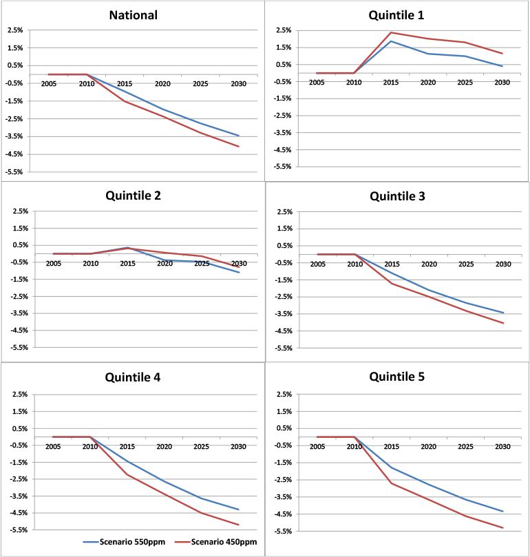
Average real net income per adult equivalent by income quintile: percentage deviations from the reference case.
Compared to the other quintiles, the lowest income quintile shows a moderate but positive impact of both mitigation scenarios. This is due to the returned permit revenue, which appears to overcompensate this group for the introduction of the mitigation policies. Indeed, the 450ppm scenario is the most favourable scenario for this quintile due to the larger lump sum transfers. Similarly, the impact of the climate-change mitigation policies is positive on the second quintile, at least initially. However, by 2020 the impact turns negative as the returned permit revenue becomes too small to compensate for reduced factor incomes.
As we move up the income distribution, this effect becomes more and more pronounced as the lump sum transfers account for a smaller share of household income (and because the share of factor income in total income increases). Hence, the reduction in income under the two mitigation scenarios is higher for individuals in the higher income quintiles, for whom factor income is much more important than benefit payments. This is an interesting result since there is a concern that lower income groups are affected more severely by climate change and by the subsequent policy changes aimed at mitigating the climate change effects, resulting in higher income inequality.
To place these results in context, Figure 2 shows the projected growth in average RNI from 2005 to 2030 for each income quintile separately. Although we should not draw any strong inferences from the predicted amounts in absolute terms, the results are useful to gain an understanding of the growth of the average RNI within each quintile relative to the other quintiles. This clearly shows that, given the assumptions that are made in the CGE and MS models, real net income growth is highest for the top quintiles but very limited for the bottom quintile. Despite the overcompensation in the two mitigation scenarios towards the lower income households, their real net income growth remains modest compared to that of the higher quintiles.
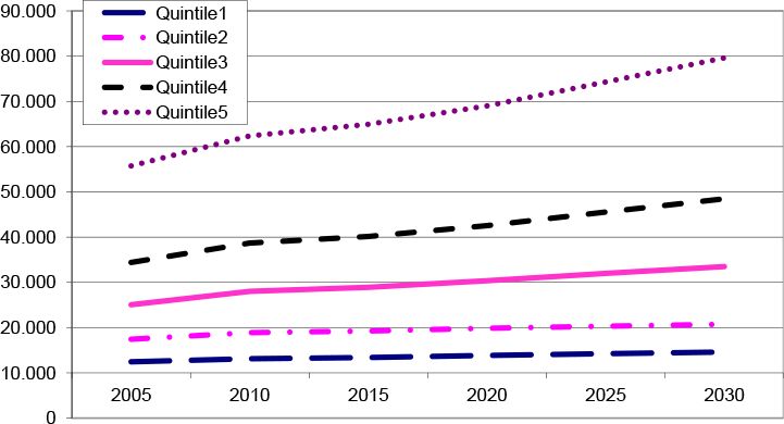
Average real net income per adult equivalent by quintile in the reference case (in financial year 2005/2006 dollars).
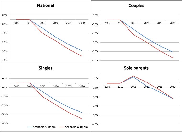
Figure 3 shows the impacts on RNI by household group. The results show some similar patterns to the results by income quintile. The largest reduction of RNI due to mitigation policies is for couple families, who also tend to be at the top end of the income distribution. Low-income households are overrepresented in the sole parents group, so similar to the lowest quintiles in Figure 1, the sole parent group appears to be better off, at least for a while, under the mitigation policy scenarios than under the reference case. Given their income sources, low-income households suffer less than other groups from slower factor income (i.e. labour plus capital income) growth while they benefit more (in relative terms) from the increasing lump sum transfers.

Average real net income per adult equivalent by household type: deviations from the reference case.
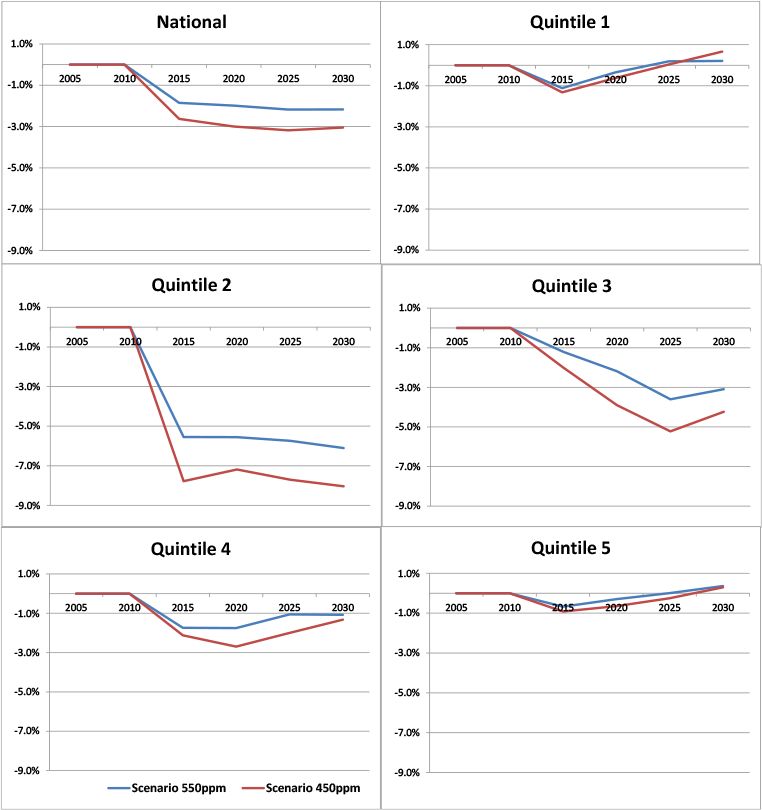
Figure 4 shows that the mitigation policies reduce income inequality, as measured by the Gini coefficient. Australia-wide, the Gini coefficient is reduced by about 3 per cent under the 450ppm scenario and by 2 per cent under the 550ppm scenario compared to the reference case. There are two main reasons for these results. First, the introduction of the ETS generates deadweight losses that are detrimental to factor income growth. Hence, factor income growth is lower under the two mitigation scenarios than under the base scenario so that the divergence between factor income and benefit payments (fixed in real terms by assumption) is reduced, and as a result inequality is reduced. Second, the lump sum transfers taking place under the mitigation scenarios have a dampening impact on inequality since they are equally distributed on a per capita basis. Should the permit revenues be returned to households in a way that targets low-income households, then inequality may be even further reduced.

Gini coefficient within income quintiles: deviations from the reference case.
As for intra-quintile inequality, the reductions are the largest for the middle quintiles whereas mitigation policies barely affect intra-group inequality for both the lowest and highest quintile. Very few of the households in the top quintile rely on benefit payments so that the reduced divergence in the growth rates of factor incomes and benefit payments would play only a minor role in reducing inequality within this group. A symmetrical explanation applies to the bottom quintile, as the share of factor income would typically be very low among this group so a decreased divergence between factor income and benefits is not so relevant either.
Figure 5 shows that both mitigation policies reduce intra-group inequality among all household groups. The lump sum transfers associated with the introduction of the ETS play a substantial role in reducing inequality in all demographic groups, and particularly among sole parents. Indeed, it is for sole parents, the lowest-income household group, that the lump sum transfers represent the largest income share and play the largest role in reducing the relative gap between working sole parents and sole parents on benefit payments, thus reducing inequality.

Gini coefficient by household type: deviations from the reference case.
5. Conclusion
This paper considers a specific approach of disaggregating output from a dynamic computable general equilibrium (CGE) model into impacts at the household and individual level. The paper draws on previous work by Robilliard et al. (2001) which linked a CGE model and an MS model in a sequential way. In this analysis, however, the CGE results had to be taken as given, and it is the MS model that is adapted to use all relevant inputs from the CGE model. This has brought problems and omissions in the CGE to the surface, showing that there would be gains to developing the two models simultaneously and making the CGE results more suitable for feeding into an MS model.
The approach used in this paper relies on altering the sample weights in order to reproduce population projections and changes in employment as predicted by the CGE model. The transmission of price changes as well as income changes from the CGE to the MS model remains similar to what can be found in the literature. That is, it relies on the transmission of average changes since CGE models only produce changes at the aggregate level. Our approach, based on adjusting sample weights, has two advantages. First, it allows the linking of an MS model to a dynamic, and not simply a static, CGE model. Second, it allows the MS model to reproduce the long-term demographic changes predicted by the CGE model (or any forecasting agency) to occur over time in the base population.
The main interest of using such an approach is that it allows the computation of the potential distributional effects of the policy change simulated in the CGE model, while explicitly accounting for the forecasted demographic changes. In this paper, the approach is applied to assess the impacts on household income of two climate-change mitigation policies compared to a reference case without mitigation. The simulations are carried out for the period from 2005 to 2030 in Australia. The results clearly show that these two mitigation policies are likely to have positive distributional effects despite a slightly negative effect on average real income. To a large extent, this is due to the redistribution of carbon permit revenues to households on a per capita basis through lump sum transfers.
Such work always involves a large number of assumptions and therefore the results that are presented should be interpreted with caution. The paper has discussed a range of important assumptions and limitations inherent to this type of modelling exercise. Ideally, the sensitivity of results to a range of assumptions should be checked before drawing any strong conclusions. A number of assumptions used in this paper were imposed by the specific CGE results used as input for the MS stage and in theory, these could be changed to be made more suitable for the distributional analysis. It is clear that the analysis could be strengthened by the simultaneous development of both models, instead of having to adapt the MS model to a given CGE model as is currently the case. For instance, the MS modelling would greatly benefit from access to aggregate results which would provide more detail on a number of key outcomes, such as for example, wage and employment changes by occupation or skill level. However, CGE modelling has its own constraints and it is not always technically feasible to generate the outcomes that are seen as crucial for MS modelling.
Despite these caveats, the results from this analysis are of interest and an important first step in setting up this type of analysis. From this analysis it appears further work would be viable and is likely to be productive. Future work could be based on alternative CGE analyses designed to capture the effects of mitigation policy changes (and associated compensation arrangements) on the income and welfare of individual households in an improved way and/or to assess the sensitivity of results to alternative assumptions.
Footnotes
1.
Chemingui and Chokri (2008) present an application to Tunisia as well as a brief literature review of other recent applications. Alternatively, the MS model can be integrated into the CGE model by increasing the number of representative households but full reconciliation between micro and macro data is then essential and the size of the model can quickly become problematic. See Cororaton and Cockburn (2007) for a recent application.
2.
In this, we extend previous work by Raihan (2010), where the linkage between the dynamic CGE model and the MS model is limited to household consumption. Bussolo et al. (2010) apply a reweighting approach similar to the one presented in this paper, although it draws on a global (and not a country-specific) CGE model and the application focuses on the effects of climate change rather than on the effects of climate change mitigation policies. A similar reweighting approach is also used by Bussolo et al. (2012) and Bussolo et al. (2011).
3.
Ferreira and Horridge (2006) present a reweighting approach to link a static CGE model to a household survey. However, it differs from the approach presented here in many aspects. See Hérault (2010) for a comparison of both approaches.
4.
See Commonwealth of Australia (2008) and the accompanying technical papers for a discussion of the CGE modelling. The main assumptions in the CGE model are summarised in Appendix A of Buddelmeyer et al. (2009).
5.
The majority of large-scale tax simulation models are non-behavioural or arithmetic. That is, no allowance is made for the possible effects of tax changes on individuals’ consumption plans or labour supplies.
6.
The latest SIHC (2005/2006) was only made available in MITTS after this research took place. Therefore, this paper is based on the 2003/2004 SIHC.
7.
For details of the different payments, see Payment Guides published by the Commonwealth Department of Family and Community Services (of several years), DVA Facts and the annual report published by the Department of Veterans’ Affairs (of several years).
8.
The survey of 2003/2004, which we use in the analysis, is uncommon in that it actually combines these two data sets, and these data would in fact be ideal to develop a consumption model together with a labour supply model. However, this combination of the two surveys will not be a regular feature; the next combined data collection occurred in 2009/2010 (ABS, 2007).
9.
See Buddelmeyer et al. (2008) for a description of the mapping process.
10.
Leaving out this adjustment would imply a substantial overestimation of factor income growth in the MS model.
11.
This is different to the current practice where allowances such as NewStart or Sickness Allowance are indexed using the CPI, but pensions, such as the Disability Support Pension, and Parenting Payment Single are indexed using wage indices (which usually increase by more than the CPI).
12.
Fixed income tax thresholds would lead to a substantial increase in the average income tax rate since real wages increase over time.
13.
Using only the budget shares of the base year is clearly unrealistic because it ignores changes in consumption patterns over time as predicted by the CGE model. In particular, it would ignore the substitution away from carbonintensive products. Using the current budget shares is not more appropriate because it would imply a ‘double counting’ of the price effects (via their effects on consumption patterns, on top of the price effects). Alternatively, average budget shares from all previous points in time could be used. The use of the budget shares from the previous point in time is preferred because it indicates who would have been most affected by a change before behaviour was adjusted.
14.
The advantage of using MS modelling is the substantial flexibility in the way the results can be broken down. In practice, the results can be broken down by any of the household characteristics available in the household survey on which the MS model is based.
15.
The weight of the first adult in each income unit is 1. The weight of each additional adult member is 0.56, and each child (under 18) is given a weight of 0.32.
16.
See Buddelmeyer et al. (2008) for an overview of these commodities and a description of the mapping of the commodities distinguished in HES into the CGE model commodities.
17.
The indexation of pensions to the wage index instead of the CPI would only have limited this problem to some extent, at the cost of an increase in the discrepancies between the CGE and the MS models.
18.
Factor income comprises labour and capital income.
19.
Similar patterns are found for the two policy scenarios. See Buddelmeyer et al. (2008) for more detail.
20.
The global financial crisis has not been taken into account in the CGE predictions, which predate the 2008 financial crisis.
21.
For each year, the values provided by the CGE model on the aggregate lump sum amounts are divided by the corresponding population sizes to obtain the lump sum transfers per capita. These per capita lump sum amounts are then added to that year’s net income of the individuals and households.
22.
Real net income is gross income plus government transfers minus income tax adjusted for inflation, using the household-specific CPIs as described in Table 1 in Section 3.2. Income units are used to construct the quintiles but each individual in the income unit is used to calculate the average real net equivalised income. For example, the bottom quintile is constructed by selecting the 20 per cent of income units who had the lowest real net income per adult equivalent, but the average real net equivalised income is based on all individuals in these 20 per cent of income units.
23.
Details of the relevant population totals are presented in Appendix D of Buddelmeyer et al. (2008).
Appendix 1. The Reweighting Procedure
The calibration approach used in this paper produces new weights which achieve specified population totals for selected variables, subject to the constraint that there are minimal adjustments to the original weights.23 The chi-squared distance function is used as the measure to minimise adjustments to the original weights.
The chi-squared type of distance measure gives the aggregate distance by:
A modification is applied to restrict the range of deviation in the revised weights (wk) from the original weights (sk). A detailed technical description of this approach can be found in Cai et al. (2006).
Table 5 summarises by how much each sample weight changes due to the reweighting procedure through reporting the size of the factor of change at each decile point of these changes. It indicates how the sample weights are affected by the reweighting procedure in the reference case. Results for the other scenarios are not reported given that they are very similar. The main reason for this similarity is that population projections are the same across scenarios and that differences in employment projections across scenarios are limited.
Ratio of new weights to original sample weights: reference case.
| 2005 | 2010 | 2015 | 2020 | 2025 | 2030 | |
|---|---|---|---|---|---|---|
| Decile 1 | 0.64 | 0.63 | 0.63 | 0.59 | 0.53 | 0.47 |
| Decile 2 | 0.77 | 0.79 | 0.82 | 0.80 | 0.77 | 0.71 |
| Decile 3 | 0.87 | 0.90 | 0.94 | 0.95 | 0.93 | 0.91 |
| Decile 4 | 0.94 | 0.99 | 1.05 | 1.09 | 1.08 | 1.07 |
| Decile 5 | 1.02 | 1.08 | 1.16 | 1.22 | 1.26 | 1.28 |
| Decile 6 | 1.10 | 1.18 | 1.27 | 1.38 | 1.42 | 1.50 |
| Decile 7 | 1.18 | 1.30 | 1.44 | 1.55 | 1.69 | 1.77 |
| Decile 8 | 1.30 | 1.45 | 1.61 | 1.77 | 1.95 | 2.15 |
| Decile 9 | 1.51 | 1.76 | 1.94 | 2.15 | 2.40 | 2.71 |
-
Note: This table should be read as follows: for 10 per cent of the records, the ratio of the new weight for 2005 (after reweighting) to the original sample weight is smaller than 0.64. For another 10 per cent of the records it is higher than 1.51.
Appendix 2. Assumptions and Limitations
This appendix provides a concise overview of a range of important assumptions that are relevant to the modelling in this paper. Due to the ‘top-down’ approach, the MS modelling inherits all the assumptions underlying the CGE model. Therefore the most relevant CGE model assumptions are listed in 2.1 before the assumptions underlying the MS analysis in 2.2. Finally, the main limitations of the modelling approach are listed in 2.3.
2.1 The CGE model (MMRF) assumptions
Treasury’s projections form the basis of the population projections underlying the CGE model.
Treasury’s projections are altered by interstate migration as predicted by the CGE model.
Employment levels by industry and region are determined by the model.
The long-run rate of unemployment is assumed to be fixed.
Changes in average wages differ by region but not by industry (nor occupation).
Base values of wages differ by region and industry (not by occupation).
63 different commodities are distinguished whose relative prices are endogenous and change over time.
Relative price changes differ by region and policy run.
Each of the eight regions has one single representative household with its own consumption function.
Adjustments in the 63 budget shares following price changes are determined at the regional level.
The same exogenous single income tax rate is applied to all representative households.
It is assumed that climate change itself will not have a direct economic impact before 2030.
Benefits from the mitigation policies resulting from a reduced adverse effect on climate will only become evident after 2030.
2.2 The MS model (MITTS) assumptions/approximations
2.2.1 The population in the MS model
The 2003/2004 Survey of Income and Housing Cost (SIHC), collected by the Australian Bureau of Statistics (2007) and uprated to the 2005/2006 financial year, is the base year file used in the MS model.
Treasury population projections are altered by the CGE model, but the CGE model does not provide information about the new age and gender structure of regional populations. A two-step reweighting approach ensures that the MS model is consistent with the CGE model and that the deviations between the MS model and Treasury projections are minimal.
The MS model is reweighted separately for every year for which a simulation is run (including base year), benchmarking the MS model input data against CGE model output to reproduce the required employment and population changes over time.
The industry classification is more aggregated in the MS model (13 industry groups) than in the CGE model (55 industry groups) thus the CGE model industries are mapped into the MS model industries.
2.2.2 Income and wages
All results are expressed in 2005/2006, or base year, prices.
Financial information in 2003/2004 is increased to reflect January 2010, 2015, 2020, 2025 and 2030 values. Non-labour income in the MS model is uprated using CGE model changes for non-labour income.
Wage rates are uprated using the average male and female wage indices until 2005, while the CGE model’s regional wage indices are used in subsequent years.
The CGE model generates average changes in wages and non-labour factor income only by region. In the MS model, the average change corresponding to the relevant region of residence is applied to each household.
2.2.3 Income tax and social security
Since the CGE model is based on the 2005/2006 financial year, the tax and social security system of January 2006 is used in the MS model.
All major social security payments and income taxes are included in the MS model.
The information in the SIHC is used to calculate eligibility for the different social security payments, not accounting for asset tests or residency requirements
Only income changes in real terms are used so that other eligibility criteria for benefits do not have to be uprated to account for inflation.
A 100 per cent take-up of benefits is assumed.
Income tax thresholds are indexed to real wages in order to hold the national average tax rate constant, in accordance with the CGE model assumptions.
Following the CGE model assumptions, all individual-benefit payments are indexed to the Consumer Price Index (CPI) in order to be held constant in real terms.
2.2.4 Income quintiles
Income quintiles are determined at the income unit level and are based on the ranking of income units according to real disposable income per adult equivalent.
Equivalising of incomes is achieved using the Whiteford equivalence scale.
New income quintiles are computed for each year of the analysis since it cannot be assumed that income units belonging to a particular quintile will still belong to the same quintile five years later.
Income quintiles differ across scenarios because changes in incomes and employment are different across scenarios.
2.2.5 Consumption behaviour
Cumulative price changes by commodity from the CGE model are combined with the previous period’s budget shares to compute real incomes adjusted for household-specific consumption patterns. using the current budget shares is not appropriate because it would imply a ‘double counting’ of the price effects (via their effects on consumption patterns, on top of the price effects).
The MS model does not include a model explaining consumption. Changes in consumption patterns as predicted by the CGE model are required as input, and this represents all behavioural responses.
In the CGE model, changes in consumption patterns are only available at the regional level and therefore the same budget share changes (in percentage points) are applied to all households’ budget shares within the same region. If these adjustments result in negative budget shares these are replaced by zero. All budget shares are evenly scaled to add up to 100 per cent following adjustment.
The 600+ expenditure items in the Household Expenditure Survey (HES) are mapped to the 63 commodities used in the CGE model.
2.3 Limitations
Changes in wages are available only at a highly aggregated level in the CGE model (changes in wages only differ by region).
The CGE model does not distinguish between skilled and unskilled workers, which is a limitation with regard to wage and employment developments.
Similarly there is no distinction in consumption responses to price changes between low and high income households.
References
-
1
MMRF-GREEN: A Dynamic Multi-Regional Applied General Equilibrium Model of the Australian Economy, Based on the MMR and MONASH ModelsMMRF-GREEN: A Dynamic Multi-Regional Applied General Equilibrium Model of the Australian Economy, Based on the MMR and MONASH Models, Draft documentation prepared for the Regional GE Modelling Course, Centre of Policy Studies, Monash university.
-
2
MMRF: A Dynamic Multi-Regional Applied General Equilibrium Model of the Australian EconomyMMRF: A Dynamic Multi-Regional Applied General Equilibrium Model of the Australian Economy, Draft documentation prepared for the Regional GE Modelling Course 16–21 July 2007, Centre of Policy Studies, Monash university.
-
3
Population Projection Australia 2004–2101Population Projection Australia 2004–2101, ABS Cat no. 3222.0..
-
4
Household Expenditure Survey and Survey of Income and Housing – Confidentialised unit Record Files. Technical Manual, Cat. No. 6540.0.00.001, CanberraHousehold Expenditure Survey and Survey of Income and Housing – Confidentialised unit Record Files. Technical Manual, Cat. No. 6540.0.00.001, Canberra.
-
5
Measures of Australia’s Progress: Summary Indicators, 2008 (Edition 2)Measures of Australia’s Progress: Summary Indicators, 2008 (Edition 2), Catalogue no. 1383.0.55.001, Canberra.
-
6
Household equivalence scales: new Australian estimates from the 1984 Household Expenditure SurveyEconomic Record 66:221–234.
-
7
Disaggregation of CGE results into household level results through micro-macro linkage: Analysing climate change mitigation policies from 2005 to 2030. Melbourne Institute Report No. 9University of Melbourne.
-
8
Linking a Dynamic CGE Model and a Microsimulation Model: Climate Change Mitigation Policies and Income Distribution in Australia. Melbourne Institute working paper no. 3/2009University of Melbourne.
-
9
Economic growth and income distribution: linking macro-economic models with household survey data at the global levelInternational journal of Microsimulation 3:92–103.
-
10
Poverty Effects of Higher Food Prices: A Global PerspectiveReview of Development Economics 15:387–402.
-
11
Global Growth and Distribution: China, India, and the Emergence of a Global Middle ClassJournal of Globalization and Development, 2, 2, Article 3.
-
12
Accounting for Population Ageing in Tax Microsimulation Modelling by Survey Reweighting. Australian Economic Papers18–37, Accounting for Population Ageing in Tax Microsimulation Modelling by Survey Reweighting. Australian Economic Papers, 45, 1.
-
13
Agricultural Trade Liberalization and Poverty in Tunisia: Micro-simulation in a General Equilibrium Framework. MPIA Working Paper 2008–03Agricultural Trade Liberalization and Poverty in Tunisia: Micro-simulation in a General Equilibrium Framework. MPIA Working Paper 2008–03.
- 14
-
15
Climate change mitigation policy modelling; Summary of assumptions and data sourcesClimate change mitigation policy modelling; Summary of assumptions and data sources, october 2008.
-
16
Trade reform and poverty – Lessons from the Philippines: A CGE-microsimulation analysisJournal of Policy Modeling 29:141–163.
-
17
Microsimulation Modelling of Taxation and The Labour Market: The Melbourne Institute Tax and Transfer SimulatorCheltenham: Edward Elgar.
-
18
Calibration estimators in survey samplingJournal of the American Statistical Association 87:376–382.
-
19
Putting Development Back into the Doha Agenda: Poverty Impacts of a WTO AgreementPutting Development Back into the Doha Agenda: Poverty Impacts of a WTO Agreement, Palgrave Macmillan and the World Bank, Washington, D.C..
-
20
Methodology for modelling climate change impacts. Technical Paper Number 4, OctoberMethodology for modelling climate change impacts. Technical Paper Number 4, October.
-
21
Sequential Linking of Computable General Equilibrium and Microsimulation Models: A Comparison of Behavioural and Reweighting TechniquesInternational Journal of Microsimulation 3:35–42.
-
22
Welfare and Poverty Impacts of Trade Liberalization: A Dynamic CGE Microsimulation AnalysisInternational Journal of Microsimulation 3:123–126.
-
23
Crisis and Income Distribution: A Micro-Macro Model for Indonesia. Technical report, International Food Policy Research InstituteWashington, D.C.
Article and author information
Author details
Acknowledgements
This paper uses CGE Modelling from the Garnaut Climate Change Review as inputs into the Melbourne Institute Tax and Transfer Simulator (MITTS) to disaggregate economy wide macro level results into results at the household and individual level. However, this work is not part of the Garnaut Report and is not endorsed by the Garnaut Review. All responsibility for the specification and outcomes of this work lies with the authors and all questions regarding this should be directed to them. However, we would like to thank Ana Markulev, Helen Morrow, Jonathan Chew, Philip Adams, Matthew Clark, Naomi Lewis, Jyothi Gali and Nicholas Stoney for their comments, suggestions and help in using the CGE output. We are also grateful to two referees and the editor for helpful comments and suggestions
Publication history
- Version of Record published: December 31, 2012 (version 1)
Copyright
© 2012, Buddelmeyer et al.
This article is distributed under the terms of the Creative Commons Attribution License, which permits unrestricted use and redistribution provided that the original author and source are credited.