
Testing the Statistical Significance of Microsimulation Results: A Plea
- Article
- Figures and data
- Jump to
Abstract
In the microsimulation literature, it is still uncommon to test the statistical significance of results. In this article we argue that this situation is both undesirable and unnecessary. Provided the parameters used in the microsimulation are exogenous, as is often the case in static microsimulation of the first-order effects of policy changes, simple statistical tests can be sufficient. Moreover, standard routines have been developed which enable applied researchers to calculate the sampling variance of microsimulation results, while taking the sample design into account, even of relatively complex statistics such as relative poverty, inequality measures and indicators of polarization, with relative ease and a limited time investment. We stress that when comparing simulated and baseline variables, as well as when comparing two simulated variables, it is crucial to take account of the covariance between those variables. Due to this covariance, the mean difference between the variables can generally (though not always) be estimated with much greater precision than the means of the separate variables.
1. Introduction
When working with sample data, testing the statistical significance of the results has become standard practice for a long time now. This is not only the case for articles in scientific journals, but also in reports of applied research for governments and other agencies. No doubt, the fact that standard errors and significance tests are routinely reported by the software packages most commonly used for this kind of empirical analysis (e.g. SAS, Stata, SPSS) plays an important role here. Also in the field of income distribution and poverty, where until recently many scientific publications ignored sampling variation, reporting standard errors and tests of statistical significance is becoming more and more common.
At the same time, tests of statistical significance are largely absent in the microsimulation literature in the field of income distribution and poverty, despite some early examples (e.g. Pudney and Sutherland, 1994). There may be a number of reasons for this situation, as discussed below. The purpose of this article is to argue that this lack of attention to statistical inference is both unnecessary and undesirable. It is structured as follows. After a discussion of the background to the current situation, we argue that straightforward statistical tests are often sufficient to assess the statistical significance of the results of specific but common types of microsimulation. Even for less straightforward situations, software is available to calculate standard errors and significance tests with little effort. We illustrate these points with results from a recent microsimulation of family benefits in Lithuania using EUROMOD, and finish with some concluding remarks regarding statistical inference in the case of more complex microsimulation studies. We stress that in this paper we are not breaking new ground in either microsimulation models or statistical inference. Rather, it is a plea to microsimulation practitioners to use the statistical tools that are at hand, in order to enhance the quality of their work.
2. Problem statement
In the light of growing budgetary pressures, there is a rising demand for comprehensive evaluations of the social impact of current versus reformed public policies, which often requires microsimulation. For example, within the field of child poverty analysis, tax-benefit microsimulation has been used to assess different (actual and hypothetical) designs of transfers to families (recent examples are Levy et al., 2009; Figari et al., 2011). The usual way of measuring the social impact of such policy options is by directly comparing point estimates (i.e. poverty measures, mean household income, total spending, etc.) derived from the original and simulated data.
Microsimulation results are subject to uncertainty. There may be uncertainty around the structure of the model (e.g., which parameters to include, the mathematical specification of the model), around the values of the model parameters, and more generally around methodological and substantive choices such as the time horizon and the measure of the outcome of interest. See Bilcke et al. (2011) for an overview of sources of uncertainty and a checklist. Sampling variability is only one of many sources of uncertainty. However, in the specific but common case of static microsimulation of the first-order impact of a reform, using a tax-benefit model without behavioural effects and sample data about actual individuals or households, sampling variability is arguably an important, if not the main source of uncertainty. The parameters in such a model are derived from official tax and benefit regulations, so there is little uncertainty around those.
When microsimulation results are based on sample data it is important to check whether these are statistically significant. Yet, perhaps surprisingly, this is not done routinely. There may be three reasons for this. First, some analysts may have the intuitive notion that sample variation does not play a role, since observed and simulated variables refer to the same sample. This notion is mistaken, because the measured effect of the simulation will depend on who is selected into the sample.
Second, some recent work on statistical inference in microsimulation has focused on changes in inequality, poverty and mobility indices, which often are non-linear functions of sample data (cf. Osier, 2009). Other authors look at statistical inference of microsimulation results where revenue-neutrality is imposed (Pudney & Sutherland, 1994) or in the case of models involving uprating to future years, behavioural relations and dynamic microsimulation (Klevmarken, 2002; Creedy et al., 2007). In addition, microsimulation models often make use of complex sample data. Until fairly recently, most analysts carried out significance tests with the implicit assumption of simple random sampling. Statisticians have always insisted that it is important to take account of the sampling design when testing the statistical significance of results (e.g. Kish, 1965; for a recent discussion see Heeringa et al., 2010) and recent papers have shown that this is also the case for poverty and income distribution studies (e.g. Howes & Lanjouw, 1998; Biewen & Jenkins, 2006; Goedemé, 2013). These studies may have created the impression that testing the significance of microsimulation results requires substantial effort from analysts, either because the analytical derivation of the sampling variance is rather complex (e.g. Pudney and Sutherland) or because bootstrapping or some other kind of time-consuming replication-based technique has to be employed (e.g. Creedy et al., 2007). However, many simulation results are simple linear functions of sample data (e.g. differences in means, sums or proportions). Calculating standard errors for those results requires only the common techniques of survey analysis and is easily done with standard software. Furthermore, over the past ten years some software packages have been developed that make it much easier for applied researchers to perform statistical tests of changes in poverty and inequality measures, while taking the sample design into account (see especially Araar & Duclos, 2007, 2009).
The third reason for the limited use of tests of statistical significance in microsimulation studies may be that most microsimulations are carried out with programs specially written for this purpose in computer languages such as Fortran and C. Commands performing significance tests are thus not readily available to microsimulators; doing such tests within these specific microsimulation packages requires either substantial programming, or the transfer of the simulated data to a statistical software package.
In order to reinforce our points, we give three examples of recent microsimulation studies on the poverty impact of diverse policy reform scenarios, where statistical tests could and should have been employed, but were not, or in a way that was less useful than was possible. In two papers no tests of statistical inference were performed at all, while in the third paper, the covariance between the baseline and reform scenario indicators was not taken into account. Sometimes the main substantive conclusions of the studies quoted below are based on microsimulation results for which the question of statistical significance is especially acute, when sample sizes are small and/or observed changes in poverty indicators are minor. The studies mentioned are diverse in terms of country coverage, policy reforms, household surveys and microsimulation model used. One of these studies (Davies & Favreault, 2004) used uprating to future years, which might complicate the calculations of correct standard errors. We come back to this issue in the section on limitations and further work.1
Davies and Favreault (2004) in their analysis of various potential US Social Security reforms, using the microsimulation model MINT3 and the Survey of Income and Program Participation conclude that “Among the limited set of reform options we consider, Social Security minimum benefit plans would be more effective in reducing poverty among low-income beneficiaries.” However, depending on the poverty measure used, differences in poverty rates between reform options were as small as 0.9 to 3.0 percentage points. No statistical tests are reported which would make it possible to evaluate which of these results, if any, are significantly different from one another. Notten and Gassmann (2008) use the Russia Longitudinal Monitoring Survey (RLMS) from 2000 to 2004 to analyse the impact of the Russian child allowance reforms and to simulate the effects of various means-tested and universal child benefit schemes. This study performs ad-hoc simulations, without any specific microsimulation model. The paper suggests that “only a significant increase of the benefit level results in considerably higher poverty reduction impacts.” These impacts are -1.9 percentage points and -5.4 percentage points. Statistical tests whether these changes are statistically significant would seem important, given the sample size of only 1079 households. In the last example, Salanauskaite and Verbist (2009) evaluate the distributional impacts of a Lithuanian family allowance reform, using EU-SILC data. The authors estimate that an initial reform would produce a 0.5 percentage point reduction in the total poverty headcount, which would increase to a 1.5 percentage points reduction if the reform would be fully implemented. They also remark that these differences are not statistically significant as indicated by the 95% confidence intervals of the pre-reform and post-reform point estimates. Apparently, these authors did not calculate the confidence intervals of the differences in the poverty headcount, which might well have been statistically significant.
3. Statistical discussion
The typical situation in static microsimulation using a tax-benefit model is that a simulated variable is compared with a corresponding variable that was observed or with another simulated variable, where both are quantitative (interval-level) variables. In many static simulations of the first-order effects of policy changes, the simulated variables are calculated using exogenous parameters (e.g. those describing a tax or benefit scheme) and possibly also observed variables (e.g. gross income). In those cases, the statistical issues are simple, as they involve a standard application of sampling theory (cf. Klevmarken, 2002: 256). It makes no difference whether an observed and a simulated variable, or two simulated variables are compared. A paired t-test can be used to assess the statistical significance of the difference of the means of the variables in the baseline and the reform scenario (Swinscow & Campbell, 2002: 71–73)2. A paired t-test takes account of the covariation between the two variables, by calculating the difference between the two variables on the individual level, and performing a one-sample t-test on the average of these differences to evaluate whether it is significantly different from zero. The equivalent of the paired t-test for qualitative (nominal) data is the equally simple but little used McNemar's test (Swinscow & Campbell, 2002: 57-59, 90-91). The necessity of taking account of the sampling design may make the calculation of tests of statistical significance considerably more complicated (e.g. Wolter, 2007; Heeringa et al., 2010), but this is also the case for any analysis of survey data. Our point is that the circumstance that we are dealing with microsimulation does not add further complications to these calculations. Furthermore, currently available software can perform this task with relatively little effort by the analyst, also in the case of distributive analyses for which freely available software packages have been developed (cf. supra).
In this discussion, we ignore 'simulation error' and potential errors introduced by uprating samples for aligning them with ‘policy years’ (see below). Simulation error is the error that is due to the fact that observed data are compared with simulated data, where the former may incorporate measurement error, and the latter may be approximations if the microsimulation model does not include all relevant tax and benefit rules (see Pudney & Sutherland, 1994 for a discussion of this issue).3
Why is it important to take the covariance into account by using the appropriate statistical tests? Recall the formula of the sampling variance (VAR) of the difference in the mean (D) of two variables y and x with means Y and X (e.g. Heeringa et al., 2010):
As becomes clear from the formula, the sampling variance of a difference does not only depend on the variance of the two estimated averages, but also on their covariance. If this covariance is strongly positive, as is usually the case for microsimulation studies, the variance of the difference of the estimated averages can be much smaller than the variance of either of the averages of the original variables y and x. If two samples are independent, then the covariance is equal to zero4. However, in the case of microsimulation studies usually two scenarios, or a scenario and the baseline, are compared based on one single sample. As a result, when comparing two scenarios, the dependence of estimates is very high and the covariance can be very strong.
Another way to present the same issue may be useful here. Suppose the variable in the baseline scenario is denoted xi, and the variable in the reform scenario is denoted yi, where the subscript i denotes the household or individual. Suppose also that the relation between xi and yi can be described by the following linear relationship:
where a and b are parameters from a microsimulation model5 Then it is easily shown that the variance of the average difference between yi and xi is equal to (capital characters indicate variable means):
Two features of this formula are noteworthy. First, the constant a does not appear, implying that the simulated result of a policy reform that increases income by the same fixed amount for every household or individual has no variance. In fact, the variance of a constant is always zero. Secondly, in the case of most policy reforms b will be positive and will be close to one. This means that the variance of D is much smaller than the variance of X, and also much smaller than the variance of Y, which (given Equation 2) is equal to b2VAR(X). For example, if b = 1.2, VAR(D) = 0.04*VAR(X) and 0.028*VAR(Y), or, in words, the variance of the difference is only 4 per cent of the variance of the mean of the original variable, and 2.8 per cent of that of the simulated variable. If simulated policy reforms combine new (increased) taxes and benefits, households will re-rank and the covariance can be much lower. However, unless the reform completely overhauls the income distribution, which any remotely plausible policy reform is unlikely to do, the covariance will not become zero or negative. This means that for policy-relevant reforms, the variance of the difference will nearly always be smaller than the variance of the difference under the assumption of having two independent samples (one before and one after the reform). This will be less true if the analysis focuses on very specific income components and/or very specific subgroups. Note also that the covariance is zero if either the original or the simulated variable is a constant value (within the subgroup). In this section, we focused on a very simple linear combination of point estimates. We would like to stress that also for non-linear combinations of point estimates (e.g. a ratio, percentage change, ...) the covariance needs to be taken into account.
4. Application using EUROMOD and Lithuanian SILC data
To illustrate the importance of estimating the sampling variance of the difference between a baseline and a reform scenario (and between various reform scenarios), we further elaborate on an example borrowed from a study by Salanauskaite and Verbist (2013). In this example we calculate the effect on mean equivalent disposable household income, poverty and inequality of a policy reform that first abolishes family benefits in Lithuania, and subsequently implements the Estonian system of family transfers. We calculate equivalent household disposable income using the modified OECD scale (cf. Atkinson et al., 2002; Decancq et al., 2013) and we simulate net disposable household income after the policy reforms using the microsimulation model EUROMOD6. We deduct gross family transfers from gross household income and recalculate net incomes by applying all relevant tax and benefit regulations to the new gross household income. Consequently, we obtain a realistic first-order estimate of net income without family transfers (respectively Estonian family transfers implemented in Lithuania), although without taking behavioural effects into account. This type of analysis is quite common in the literature, and issues regarding variance estimation are not different from those when estimating the effect of many other, more complicated policy reforms. Below we discuss cases in which variance estimation is less straightforward.
In this illustration we use Lithuanian data, which are derived from the EU-SILC 2006 survey (Ivaškaitė-Tamošiūnė et al., 2010). The income reference year is 2005 and the analysed policy year is 2008. As the income reference date is “older” than analysed policies, EUROMOD utilises a number of country-specific adjustment factors to update income levels to the corresponding policy year7. The chosen data and policy years are aligned with the assumptions of the Salanauskaite and Verbist (2013) study, where this as well as other examples of microsimulation reform scenarios are discussed in more detail.
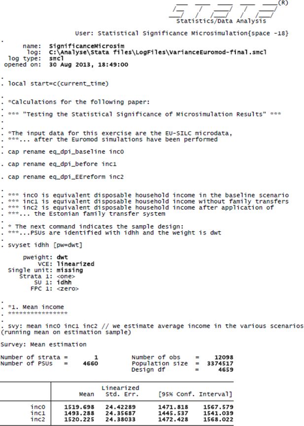
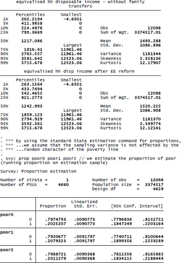
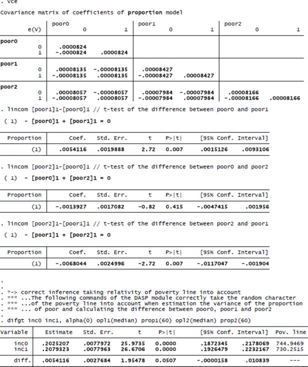
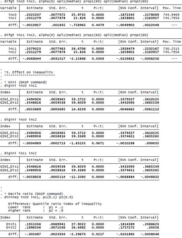
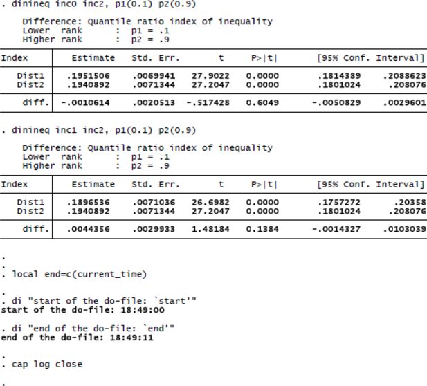
The Lithuanian sample contains information on 12,098 individuals and 4,660 households.8 The Lithuanian EU-SILC sample has a single-stage stratified sample design. Within each of the seven strata a simple random sample of persons is drawn and the entire household of each selected person is included in the sample (Statistics Lithuania, 2010). Therefore, we take account of clustering at the household level, but unfortunately we lack information on stratification in the data. As a result, the standard errors are likely to be slightly over-estimated (e.g. Kish, 1965). All variance estimates are based on Taylor first order linearization and make use of Stata standard estimation procedures and the DASP module developed for Stata (Duclos & Araar, 2006; Araar & Duclos, 2007)9. The advantage of DASP is that it includes standard estimation commands for typical distributive analyses in relation to poverty, inequality and polarization. DASP is also available as a stand-alone free software package under the name of DAD (Araar & Duclos, 2009). For all statistical tests presented below, we made use of ready-made routines that require very little effort in programming and in computation time. Once all income variables are prepared, running the computations for the results presented in the table below takes less than 15 seconds with Stata/SE 11.210.
Our estimates presented in Table 1 illustrate the two points to which we have drawn attention in the previous sections. First of all, the variance of point estimates cannot be ignored as even for estimates on the basis of a relatively large sample standard errors and confidence intervals are quite substantial. Second, it is crucial to take the covariance between the baseline scenario and the reform scenario into account: not doing so would result in a very misleading interpretation of the statistical significance of the simulated distributive effects of reforms.
The effect of family transfers on equivalent disposable household income in Lithuania, EU-SILC 2006.
| Panel / Outcome | 95% confidence interval | ||||
|---|---|---|---|---|---|
| Scenario | Estimate | Standard-error | Lower bound | Upper bound | |
| (A) Mean equivalent income | Baseline (1) | 1,519.70 | 24.42 | 1,471.82 | 1,567.58 |
| Without family transfers (2) | 1,493.29 | 24.36 | 1,445.54 | 1,541.04 | |
| Estonian family transfers (3) | 1,520.23 | 24.38 | 1,472.43 | 1,568.02 | |
| Difference (2)–(1) | −26.41 | 0.86 | −28.11 | −24.71 | |
| Difference (3)–(1) | 0.53 | 0.45 | −0.35 | 1.41 | |
| Difference (3)–(2) | 26.94 | 0.99 | 25.00 | 28.88 | |
| (B) Percentage poor (fixed poverty line) | Baseline (1) | 20.25 | 0.91 | 18.47 | 22.03 |
| Without family transfers (2) | 21.57 | 0.93 | 19.75 | 23.39 | |
| Estonian family transfers (3) | 20.08 | 0.90 | 18.30 | 21.85 | |
| Difference (2)–(1) | 1.32 | 0.26 | 0.81 | 1.83 | |
| Difference (3)–(1) | −0.18 | 0.17 | −0.51 | 0.16 | |
| Difference (3)–(2) | −1.49 | 0.30 | −2.08 | −0.91 | |
| (C) Percentage poor (floating poverty line) | Baseline (1) | 20.25 | 0.78 | 18.72 | 21.78 |
| Without family transfers (2) | 20.79 | 0.78 | 19.26 | 22.32 | |
| Estonian family transfers (3) | 20.11 | 0.78 | 18.59 | 21.64 | |
| Difference (2)–(1) | 0.54 | 0.28 | −0.00 | 1.08 | |
| Difference (3)–(1) | −0.14 | 0.18 | −0.50 | 0.22 | |
| Difference (3)–(2) | −0.68 | 0.32 | −1.30 | −0.06 | |
| (D) Gini coefficient | Baseline (1) | 34.95 | 0.59 | 33.79 | 36.11 |
| Without family transfers (2) | 35.49 | 0.60 | 34.32 | 36.66 | |
| Estonian family transfers (3) | 34.90 | 0.59 | 33.75 | 36.05 | |
| Difference (2)–(1) | 0.54 | 0.04 | 0.47 | 0.61 | |
| Difference (3)–(1) | −0.05 | 0.03 | −0.10 | 0.00 | |
| Difference (3)–(2) | −0.59 | 0.05 | −0.69 | −0.49 | |
| (E) Decile ratio | Baseline (1) | 19.52 | 0.70 | 18.14 | 20.89 |
| Without family transfers (2) | 18.97 | 0.71 | 17.57 | 20.36 | |
| Estonian family transfers (3) | 19.41 | 0.71 | 18.01 | 20.81 | |
| Difference (2)–(1) | −0.55 | 0.24 | −1.02 | −0.08 | |
| Difference (3)–(1) | −0.11 | 0.21 | −0.51 | 0.30 | |
| Difference (3)–(2) | 0.44 | 0.30 | −0.14 | 1.03 | |
-
Notes: The poverty line is calculated as 60 per cent of the median equivalent disposable household income. In the case of a fixed poverty line, the poverty line is kept constant for incomes with and without family transfers. In the case of a floating poverty line, the poverty line is equal to 60 per cent of the median equivalent disposable household income, with the median income recalculated in every reform scenario.
Source: EU-SILC 2006 UDB, EUROMOD, own calculations. Results in panels A and B are calculated with standard Stata commands, those in panels C, D and E with the DASP module. See the Appendix for details.
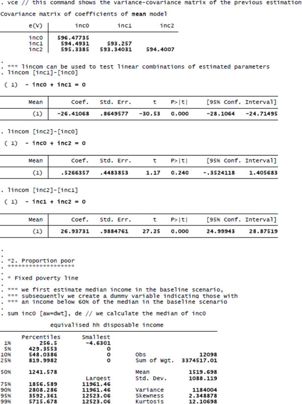
Panel A shows average equivalent disposable household income in the baseline scenario and the two reform scenarios (the first three rows), as well as a t-test of the difference between mean income in the three scenarios (the subsequent three rows shaded in grey). For all three income definitions the width of the 95% confidence interval is close to 100 EUR. The 95% confidence intervals considerably overlap: for average income in the baseline and in the third scenario it ranges from 1472 EUR to 1568 EUR and for average income without family transfers it ranges between 1446 EUR and 1541 EUR. The finding that the confidence intervals overlap does not imply, though, that abolishing family transfers (scenario 2) has no significant effect on average equivalent disposable household. The fourth and sixth row clearly show that even though average income has decreased by just over 26 EUR when the baseline and the second scenario are compared, this difference is highly significant, with the 95% confidence interval being only 3 EUR wide. The effect on average incomes can be estimated with a high degree of precision even though the confidence intervals around average incomes are rather substantial. This is because the covariance between mean income in the baseline and in the reform scenario is so strong: it is equal to 594.5, corresponding to a correlation coefficient of 0.9995. This is a clear illustration of the importance of taking account of the covariance, as discussed above. Note that we would come to exactly the same conclusion if we would calculate first for each person or household individually the difference between income in the reform and in the baseline scenario and subsequently estimate the confidence interval of the average of the difference11. The simulation of the Estonian family benefit system (scenario 3) does not produce a significant effect (on average, results not shown here indicate that there are significant changes in mean income for several subpopulations). Nonetheless, we include this scenario in the example to show that it is also easy to compute standard errors and confidence intervals for the differences between two reform scenarios. On the basis of the sixth row, it can be seen that the implementation of Estonian family benefits in Lithuania would lead to a significant increase in average equivalent disposable household income compared to reform scenario 2. Also in this case, a strong covariance exists between mean income in the two reform scenarios.
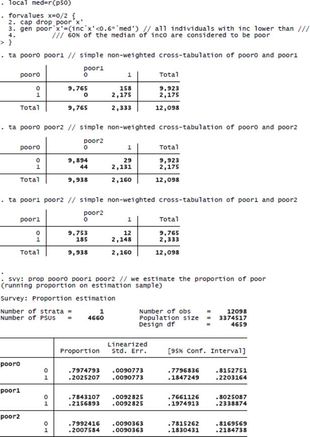
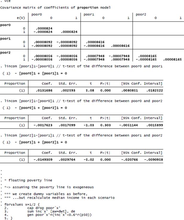
The same observation holds true for the proportion of individuals living in a household with an equivalent disposable household income below the poverty threshold. In panel B the poverty threshold is equal to 60 per cent of median equivalent disposable household income in the baseline scenario, but it is assumed to be exogenous and not subject to sampling variance. When family transfers are deducted, the poverty rate rises from 20.2 to 21.6 per cent of the Lithuanian population. Here again, it is clear that even though 95% confidence intervals of both percentages considerably overlap, the difference between them is strongly significant, with the standard error of the difference being much smaller than the standard error of the estimated percentages in poverty. In contrast, if we assume a floating poverty line, calculated at 60 per cent of the median equivalent (simulated) household income, we can observe from panel C that the difference between the various scenarios is smaller and no longer significant. In fact, taking account of the sampling variance of the poverty threshold tends to reduce the standard error of the poverty headcount (for an explanation, see Preston, 1995; Berger & Skinner, 2003; Goedemé, 2012), but leads in our illustration to larger standard errors for differences between poverty headcounts.
The conclusions for more complex, ‘non-smooth’ inequality indicators such as the Gini coefficient (panel D) and the ratio of the tenth and the ninetieth percentile (i.e. the decile ratio; panel E) are similar to those for the change in average income: even though the sampling variances of estimated inequality measures are non-negligible, the difference between inequality in the baseline scenario and the reform scenarios (and between both reform scenarios) can be estimated with a high degree of precision. Please note that for some reforms the covariance may be much smaller (this could be the case if a large amount of re-ranking takes place), so that even larger differences between the baseline and simulated scenarios could be non-significant.
5. Limitations and further work
In this article we have argued that standard survey methods and techniques are in specific but common cases sufficient to calculate standard errors and confidence intervals for microsimulation results. Those specific cases are static microsimulations of the first-order impact of a reform, using a tax-benefit model without behavioural effects and sample data about actual individuals or households. In such applications of microsimulation models, sampling variability is arguably an important, if not the main source of uncertainty. However, even such studies may have features which complicate matters.
For instance, the policy year of interest and the income reference year of the underlying database may differ, involving the need to ‘uprate’ the database (see e.g. Ivaškaitė et al., 2010). This may be accomplished by changing the weights to adjust the composition of the sample, and by multiplying incomes and other amounts by exogenously given coefficients. If the weights are adapted to reflect the distribution as found in another source that is not subject to sampling variance, weights are similar to poststratification weights, and are easily handled by current statistical software (cf. Heeringa et al., 2010). Adjusting incomes by multiplying them with a fixed factor is similar to what happens routinely in tax-benefit models, and its effects on standard errors and confidence intervals are also automatically taken into account by standard statistical techniques and software. However, other forms of uprating may present bigger difficulties that warrant further investigation in terms of the most accurate and efficient method for estimating the sampling variance. For instance, instead of multiplying certain incomes with a fixed factor, they may be aligned with external sources such that the total income reflects national accounts estimates. In addition, some uprating factors may be based on other sample survey estimates, which adds an additional, independent source of random error.
Another difficult case are microsimulations using budget-neutral scenarios, where the size of the benefits in the reform scenario is adjusted so that their total matches total expenditure in the baseline scenario (e.g. Clauss & Schubert, 2009; Levy et al., 2009; Salanauskaite & Verbist, 2013). This induces dependence between the baseline and the reform scenario that could affect the covariance in an unpredictable way. The same is true for estimating the effect of reform scenarios in a dynamic model that incorporates behavioural effects, or any other reform that includes some stochastic element (e.g. Immervoll et al., 2007; Ericson & Flood, 2012; Navicke et al., 2013; for a survey of techniques applied in dynamic modelling, see Li & O’Donoghue, 2013). Future research could assess whether, for instance, bootstrapping the effect would result in an accurate estimate of the sampling variance and whether more naive estimates of the variance, ignoring this dependence, result in strongly biased variance estimates or not. Previous papers have already addressed parts of these questions (e.g. Pudney & Sutherland, 1994, 1996; Klevmarken, 2002; Creedy et al., 2007), but have so far not resulted in universally applicable solutions and user-friendly software. The same is true for testing the impact of monte-carlo variance in dynamic simulations, i.e. the variance induced by randomly sampled model inputs; cf. O’Hagan et al. (2007). More research is needed for estimating the confidence intervals of the effects of more complex simulations, and especially the development of software to enable microsimulation practitioners to perform proper statistical tests for complex analyses with relative ease. Our discussion is limited to microsimulation studies in the field of income distribution and poverty. In other fields, such as health, microsimulation practitioners seem to have greater awareness of statisticial issues of uncertainty and accuracy. See, for example, O’Hagen et al. (2007) and Sharif et al. (2012). Cross-field exchange of techniques and methods might be of great benefit.
6. Concluding remarks
As we have shown in this article, the sampling variance cannot be ignored in microsimulation studies of poverty and inequality, working with sample data. In many situations, sampling variance is an important source of uncertainty, and standard statistical techniques suffice to perform the appropriate test of significance (though the sample design may complicate matters). Furthermore, standard routines have been developed which make it possible for applied researchers to calculate the sampling variance, while taking the sample design into account, of relatively complex statistics such as relative poverty, inequality measures and indicators of polarization, with relative ease and a limited time investment. Very helpful in this regard, is the software developed at the Université Laval (Duclos & Araar, 2006; Araar & Duclos, 2007, 2009). Therefore, we would like to encourage practitioners of microsimulation to use these routines and to estimate and report standard errors and confidence intervals for their results. As Klevmarken (2002: 264) has written "The credibility of [microsimulation models] with the research community as well as with users will in the long run depend on the application of sound principles of inference in the estimation, testing and validation of these models."
At the same time however, we would like to stress that when comparing baseline and reform scenarios, as well as when comparing two reform scenarios, it is crucial to take account of the covariance which will generally, though not always, result in a high degree of precision of estimates of the effect of a reform, even though the sampling variance of the separate point estimates may be substantial. Furthermore, also the characteristics of the indicator of interest and the structure of the sample design should be properly taken into account.
We have also noted that many microsimulation studies involve complex estimation procedures, where application of standard techniques and software does not necessarily produce the correct standard errors. However, this cannot be an excuse for not making and reporting tests of statistical significance. Reporting a less than ideal test (and mentioning the shortcomings) is still far better than totally ignoring sampling variability and other sources of uncertainty. While new research is necessary to develop user-friendly software and procedures that can accommodate more complex problems, microsimulation researchers could and should make use of the user- friendly software for statistical tests that is already available to them.
Footnotes
1.
In taking these three studies as examples, we do not want to target special criticism to the authors. We have chosen these papers because they are typical (competent and interesting) applications of static microsimulation.
2.
We refer purposefully to this very good but also very introductory text in order to underline our point that in the situations indicated the most basic of statistical techniques are sufficient to perform the appropriate tests of significance (disregarding complications introduced by the sampling design).
3.
Simulation error and measurement error are of a rather different kind than sampling error. The latter is the consequence of the random selection of a limited number of sample units from a larger population, while the first refer to a difference between the measured or simulated value of a particular observation and its real value in some sense. In ignoring simulation and measurement error we follow current practice in inferential statistics in survey analysis. This does not mean that such error does not have an impact on the estimated standard errors and significance levels, but the size and direction of the impact depend on the kind of error and the assumptions that are made regarding its properties. In general, a source of variation that affects one variable but not another one, will reduce the covariance between those variables (and thus increase the standard error of the average difference of those variables). If the baseline variable is directly observed, while the reform scenario variable is simulated using tax-and-benefit rules only, measurement error will only be present in the former variable, reducing the covariance between the baseline and reform scenario variables. On the other hand, if both variables are simulated with the same microsimulation model, any simulation error in those variables is likely to be correlated, possibly increasing the covariance between the two variables. unless the simulation error has the convenient but unlikely properties of zero mean and no correlation with true values, the standard error of the average difference (as well as the average difference itself) could be biased. A full discussion of these issues is far outside the scope of this paper.
4.
As has been stressed also in other fields of study: simply checking whether confidence intervals do not overlap in the case of independent samples is overly conservative. This is because VAR(X)^0.5 plus VAR(Y)^0.5 is larger than (VAR(X) + VAR(Y))^0.5. If confidence intervals are compared then the former formula (multiplied with a t-value) is applied, even though, as explained above, the second formula is the correct one (cf. Schenker and Gentleman, 2001; Wolfe and Hanley, 2002; Afshartous and Preston, 2010; Cumming, 2009).
5.
It is important that the coefficients a and b are not interpreted as sample estimates (e.g. least- square estimates), since that would imply that they are not exogenously given.
6.
The used EUROMOD version is F3.0. More details on the EUROMOD model are available in e.g. Sutherland and Figari (2013). More information on the simulation of Lithuanian policies in EUROMOD is available in Ivaškaitė-Tamošiūnė et al. (2010).
7.
In some cases this may also influence the sampling variance. However, in this article we focus on the principal sources of the sampling variance that can relatively easily be taken into account. Further research is necessary to evaluate how various forms of uprating can most easily be taken into account and to estimate what their potential impact is on the sampling variance.
8.
In comparison to the original EU-SILC data, observations of 36 children born in the year of survey collection are dropped. Information on newborns in 2006 is actually available only until the survey collection time (May-June, 2006). By dropping this group, we align income and demographic references to the calendar year of 2005.
9.
10.
Given the illustrative nature of our empirical results, and the fact that we use software that is easily available, we do not present the formulas used. These can be found in the literature referred to, in particular Heeringa et al♦. (2010) and StataCorp (2011) for the standard errors and confidence intervals reported in panels A and B of Table 1 and Duclos and Araar (2006) for the results reported in panels C, D and E.
11.
In fact, this is the way that Stata calculates a paired t-test (StataCorp, 2009: 2002).
7. Appendix: stata® code and output
References
-
1
Confidence intervals for dependent data: Equating non-overlap with statistical significanceComputational Statistics & Data Analysis 54:2296–2305.
-
2
DASP: Distributive Analysis Stata Package: PEP, CIRPÉE and World BankUniversité Laval.
-
3
DAD: A Software for Poverty and Distributive AnalysisJournal of Economic & Social Measurement 34:175–189.https://doi.org/10.3233/JEM-2009-0315
- 4
-
5
Variance Estimation for a Low Income ProportionJournal of the Royal Statistical Society. Series C (Applied Statistics) 52:457–468.
-
6
Variance Estimation for Generalized Entropy and Atkinson Inequality Indices: the Complex Survey Data CaseOxford Bulletin of Economics and Statistics 68:371–383.
-
7
Accounting for Methodological, Structural, and Parameter Uncertainty in Decision-Analytic Models: A Practical GuideMedical Decision Making 31:675–692.https://doi.org/10.1177/0272989x11409240
-
8
Microsimulation meets general equilibruim - a new tool for applied policy analysisIn: A Zaidi, A Harding, P Williamson, editors. New Frontiers in Microsimulation Modelling. Surrey: Ashgate. pp. 557–580.
-
9
Confidence intervals for policy reforms in behavioural tax microsimulation modellingBulletin of Economic Research 59:37–65.https://doi.org/10.1111/j.0307-3378.2007.00250.x
-
10
Inference by eye: Reading the overlap of independent confidence intervalsStatistics in Medicine 28:205–220.https://doi.org/10.1002/sim.3471
-
11
Interactions between social security reform and the supplemental security income program for the aged, Center for Retirement Research working paper, 2004–02Chestnut Hill, MA: Center for Retirement Research at Boston College.
-
12
The Evolution of Poverty in the European Union: Concepts, Measurement and Data, ImPRovE Methodological paper 13/01Antwerp: Herman Deleeck Centre for Social Policy, University of Antwerp.
- 13
-
14
A Microsimulation Approach to an Optimal Swedish Income TaxInternational Journal of Microsimulation 5:2–21.
-
15
Measuring the Size and Impact of Public Cash Support for Children in Cross-National PerspectiveSocial Science Computer Review 29:85–102.
-
16
Essays on poverty and minimum income protection for Europe's elderly262p, Essays on poverty and minimum income protection for Europe's elderly, PhD dissertation, Antwerp, University of Antwerp.
-
17
How much confidence can we have in EU-SILC? Complex sample designs and the standard error of the Europe 2020 poverty indicatorsSocial Indicators Research 110:89–110.https://doi.org/10.1007/s11205-011-9918-2
- 18
-
19
Does Sample Design Matter for Poverty Rate Comparisons?Review of Income & Wealth 44:99–109.
-
20
Welfare reform in European countries: a microsimulation analysisThe Economic Journal 117:1–44.https://doi.org/10.1111/j.1468-0297.2007.02000.x
- 21
- 22
-
23
Statistical inference in micro-simulation models: incorporating external informationMathematics and Computers in Simulation 59:255–265.https://doi.org/10.1016/S0378-4754(01)00413-X
-
24
Alternative Tax-Benefit Strategies to Support Children in PolandIn: O Lelkes, H Sutherland, editors. Tax and Benefit Policies in the Enlarged Europe: Assessing the Impact with Microsimulation Models. Surrey: Ashgate. pp. 125–152.
-
25
A survey of dynamic microsimulation models: uses, model structure and methodologyInternational Journal of Microsimulation 6:3–55.
-
26
Nowcasting Indicators of Poverty Risk in the European Union: A Microsimulation ApproachSocial Indicators Research, online first: 1-19, 10.1007/s11205-013-0491-8.
-
27
Size matters: targeting efficiency and poverty reduction effects of means-tested and universal child benefits in RussiaJournal of European Social Policy 18:260–274.https://doi.org/10.1177/0958928708091059
-
28
Monte Carlo probabilistic sensitivity analysis for patient level simulation models: efficient estimation of mean and variance using ANOVAHealth Economics 16:1009–1023.
-
29
Variance Estimation for Complex Indicators of Poverty and Inequality Using Linearization TechniquesSurvey Research Methods 3:167–195.
-
30
Sampling Distributions of Relative Poverty StatisticsJournal of the Royal Statistical Society. Series C (Applied Statistics) 44:91–99.
-
31
How reliable are microsimulation results? An analysis of the role of sampling error in a U.K. tax-benefit modelJournal of Public Economics 53:327–365.
-
32
Statistical Reliability in Microsimulation Models with Econometrically-Estimated Behavioural ResponsesIn: A Harding, editors. Microsimulation and Public Policy. Bingley: Emerald Group Publishing Limited. pp. 453–472.
-
33
Reforming Child Allowances in Lithuania: What Does Microsimulation Tell Us?In: O Lelkes, H Sutherland, editors. Tax and Benefit Policies in the Enlarged Europe: Assessing the Impact with Microsimulation Models. Surrey: Ashgate. pp. 139–170.
-
34
Is the Neighbour's Grass Greener? Comparing Family Support in Lithuania and Four Other New Member StatesJournal of European Social Policy 23:315–331.
-
35
On Judging the Significance of Differences by Examining the Overlap Between Confidence IntervalsThe American Statistician 55:182–186.https://doi.org/10.1198/000313001317097960
-
36
Uncertainty Analysis in Population-Based Disease Microsimulation ModelsEpidemiology Research International, 2012(Article ID 610405) pp. 1–14.https://doi.org/10.1155/2012/610405
- 37
-
38
Stata Base Reference Manual Release 122392p, Stata Base Reference Manual Release 12, College Station, TX, Stata Press.
- 39
-
40
EUROMOD: the European Union tax-benefit microsimulation modelInternational Journal of Microsimulation 6:4–26.
- 41
-
42
If we’re so different, why do we keep overlapping? When 1 plus 1 doesn't make 2CMAJ: Canadian Medical Association Journal 166:65–66.
- 43
Article and author information
Author details
Acknowledgements
We are grateful to Paola De Agostini, Jekaterina Navicke, Iva Tasseva, Holly Sutherland, the participants of the workshop at the 3rd ImPRovE meeting in Urbino (http://improve-research.eu), 3 May 2013, the participants at the 2013 EUROMOD research workshop & project meeting at Lisbon on 2–4 October 2013, the editor and two anonymous referees for very helpful comments and suggestions. This research benefited from financial support of the European Union's Seventh Framework Programme (FP7/2012–2016) under grant agreement n° 290613 within the project Poverty Reduction in Europe: Social Policy and Innovation (ImPRovE, http://improve-research.eu), funding of IWT-Flanders in the framework of the SBO-project “FLEMOSI: A tool for ex ante evaluation of socio-economic policies in Flanders” (www.flemosi.be) as well as funding from the Flemish ‘Methusalem’ programme. The views expressed in this paper do not necessarily correspond to those of the funding agencies. All remaining errors and shortcomings are our own.
Publication history
- Version of Record published: December 31, 2013 (version 1)
Copyright
© 2013, Goedemé
This article is distributed under the terms of the Creative Commons Attribution License, which permits unrestricted use and redistribution provided that the original author and source are credited.

