Imputing individual effects in dynamic microsimulation models an application to household formation and labour market participation in Italy
- University of Oxford Nuffield College, United Kingdom
- Collegio Carlo Alberto and LABORatorio Revelli, Italy
- LABORatorio Revelli, University of Milan-Bicocca, Italy
- Article
- Figures and data
-
Jump to
- Abstract
- 1. Introduction
- 2. Unobserved heterogeneity and dynamic microsimulations
- 3. The Rank method
- 4. Female labor supply in Italy
- 5. Data, econometric specifications and estimation results
- 6. The microsimulation model
- 7. Model comparison and validation
- 8. Conclusions
- Footnotes
- References
- Article and author information
Abstract
Dynamic microsimulation modelling involves two stages: estimation and forecasting. Unobserved heterogeneity is often considered in estimation, but not in forecasting, beyond trivial cases. Non-trivial cases involve individuals that enter the simulation with a history of previous outcomes. We show that the simple solutions of attributing to these individuals a null effect or a random draw from the estimated unconditional distributions lead to biased forecasts, which are often worse than those obtained neglecting unobserved heterogeneity altogether. We then present a first implementation of the Rank method, a new algorithm for assigning individual effects to the simulation sample. Out-of-sample validation of our model shows that use of the Rank method significantly improves the quality of the forecasts.
1. Introduction
In dynamic microsimulation models, the dynamics of each process are generally governed by coefficients that have been estimated on historical data. The choice of the econometric specification is therefore crucial for the quality of the predictions. This is particularly true when unobserved heterogeneity (UH) is an issue, given that microsimulations have been explicitly developed to allow distributional analysis and hence a thorough consideration of individual idiosyncrasies. However, netting out the estimated coefficients from the effects of individual-specific components does not guarantee better quality forecasts, as long as these individual-specific components are not appropriately simulated. This is an easy task if the simulation sample is the same as the estimation sample (statistical packages generally provide an estimation of the individual effect for each estimation unit), or if “new” simulated individuals enter the simulation without a history of previous outcomes (the individual effects can be randomly assigned by drawing from their estimated unconditional distributions). If this is not the case, individual effects should be drawn from conditional (posterior) distributions, given the observed outcomes and the value of the covariates.
As an example, suppose that a model of labour market participation (a 0–1 process) has been estimated on panel data by means of a probit model with random effects. This means that some individuals have a higher probability of participation thanks to unobservable characteristics, say motivation, attitude, etc. We get estimates for the coefficients, and an estimate for the standard deviation of the random effects, which are assumed to be normally distributed and independent of the observables. We want to apply these estimates to a different population, which is observed in the base year. This means –let us be redundant at this point– that in the base year we observe the observables, and we do not observe the unobservable characteristics of our population. Shall we simply ignore the unobservables, or shall we impute a random effect to each individual in the simulation sample? Take two individuals with the same observable characteristics: individual A is active, while individual B is inactive. Clearly, it is more likely that A has more favourable unobservable traits than B. If we ignore UH, the simulated labour market trajectories of A and B will be a priori similar, and heterogeneity is lost. If we sample from the estimated (unconditional) normal distribution of the individual effects, there is an equal probability that A gets a less favourable individual effect than B, or B gets a less favourable individual effect than A, which is also incorrect. The individual effect for A must be sampled from a different distribution than the one used for B.
Unfortunately, except in the linear case with Gaussian disturbances, sampling from posterior distributions requires the repeated application of numerical integration methods, which may be computationally demanding. A different strategy has therefore emerged, which consists in drawing all individual effects from their unconditional distributions, and then assigning each random draw to a simulated individual with the aim to minimize an overall distance between realized and simulated outcomes (Panis, 2003). This optimal assignment approach however runs into two problems: first, it introduces, in nonlinear models, a correlation between the individual effects and the covariates. Second, it is also computationally burdensome: the available optimal assignment algorithms developed in the operations research literature work in polynomial time (Carpaneto et al., 1988; Burkard et al., 2008). Richiardi (2014) develops an algorithm that provides an optimal solution to the assignment problem in linear regression models, and an approximation of the optimal solution in nonlinear (binary response) models.1 This approximation has two interesting features: it greatly reduces the induced correlation problem of the optimal assignment solution in binary response models, and it is much faster, working in quasi-linear (N log N) time.
In this paper we test this method vis-à-vis the standard approaches for dealing with UH in dynamic microsimulation models. Specifically, we compare the outcomes in terms of participation rates of different subgroups of the population in four versions of a microsimulation model: a benchmark in which all processes are modelled by means of simple pooled probit specifications with lagged endogenous variables and no UH, and three alternatives in which we specify random effect dynamic probit models, where initial conditions are estimated following Heckman (1981a, 1981b). These three variations differ in how individual UH is imputed in the simulated population: in the first one we assign an individual effect equal to zero (a “null” effect) to all individuals, in the second one we assign each individual a random draw from the estimated unconditional distribution of UH, while in the third one we use the Rank method to assign each individual a random draw that matches his or her observed past history. We show that the differences in projected outcomes are large and significant. We base our estimations on the complete series of the European Community Household Panel (ECHP), which runs from 1994 to 2001, in order to be able to perform out-of-sample validation in the subsequent years. We find evidence that the forecasts obtained with imputation of UH through the Rank method remain sensibly more on track with historical data. Our microsimulation is applied to Italian data: for the purpose of our work, this is a particularly apt case study, as female participation rates are still very low as compared to other EU countries, despite having markedly increased over the past decades (Del Boca et al., 2006). This leaves space for a further increase (Leombruni and Richiardi, 2006), and makes the outcome of the microsimulation highly sensitive to the estimated coefficients.
The paper is structured as follows. Section 2 discusses the methodological problem that motivates our analysis; Section 3 describes in more details the Rank method; Section 4 describes the evolution and the main determinants, according to the literature, of female labour force participation in Italy, and elaborates on why this is an interesting testbed for our exercise; Section 5 discusses the econometric specifications and estimates; Section 6 describes the microsimulation model; Section 7 presents our out-of-sample validation of the different imputation methods; Section 8 wraps up and concludes.
2. Unobserved heterogeneity and dynamic microsimulations
Microsimulation models often consider dichotomous processes, e.g. labour market participation, household formation, fertility. They are generally modelled by comparing the value of a latent outcome variable y*, assumed to be a function of observable characteristics of the individual, with a threshold.2 In the case of a probit
which gives raise to the standard expression
where Φ is the cumulative distribution function of a standard normal distribution, x is a vector of strictly exogenous observed explanatory variables for individual i at time t, and the vector β contains the parameters to be estimated.
Often, these processes are characterized by a high degree of persistence, i.e. the explanatory power of lagged dependent variables is very high. Including the lagged dependent variable in this settings leads to
with γ being an additional parameter to be estimated.3
This poses no problems if observed persistence is only due to true state dependence. In this case, being in a certain state (e.g. participate to the labour market) in a specific time period, in itself, increases the probability of being in the same state in subsequent periods. However, observed persistence may also be due to permanent UH:4
where αi indicates the individual-specific effect.
According to equation (4), individuals are heterogeneous with respect to characteristics that are relevant for the chance of being (and remaining) in a certain state. For example, an individual might participate to the labour market despite unfavourable observable characteristics, due to favourable unobservable characteristics like a special taste for work, work ethics, need for money etc. These characteristics are likely to be at least to some extent persistent over time; therefore, they increase the likelihood that the individual will also participate in the future. These unobserved individual effects work in every respect as omitted variables. As Wooldridge (2005a, p. 27) puts it, “[i]n nonlinear models, much has been made about the deleterious effects that ignoring heterogeneity can have on the estimation of parameters, even when the heterogeneity is assumed to be independent of the observed covariates. A leading case is the probit model with an omitted variable. Yatchew and Griliches (1985) show that when the omitted variable is independent of the explanatory variables and normally distributed, the probit estimators suffer from (asymptotic) attenuation bias. This result is sometimes cited to illustrate how a misspecification that is innocuous in linear models leads to problems in nonlinear models”.5 Moreover, the individual effect is not independent of the lagged dependent variable, if included among the covariates, as the latter is correlated by construction with the lagged residual, which includes the unobserved permanent individual effect. As a result, estimates of state dependence that fail to account for permanent UH are in general upward biased: the model attributes to true state dependence any individual effect that makes a transition to a different state less likely.6
Most microsimulation models now take into account UH, at least in the core processes under study.
However, when simulation is involved an additional problem arises, concerning the imputation of the individual effects to the simulated individuals. This is less of an issue in static microsimulations, as the simulation sample generally coincides with the estimation sample, where individual effects can be estimated. On the other hand, dynamic microsimulations generally include many processes (like schooling, household formation, labour market transitions, retirement, etc.): it is quite unlikely that a single dataset exists with all the relevant variables so that it can be used both for estimation of all processes and as a basis for simulation; this being all the more so as models with UH require panel data for estimation. A more common situation is to estimate different processes on different datasets, and then apply the estimated coefficients to some initial population to be simulated forward in time. Moreover, the initial population generally needs to be expanded as the simulation proceeds, possibly including offspring, spouses and immigrants. If the simulated individuals enter the simulation without a history of previous outcomes, the solution is straightforward: sampling random individual effects from the estimated (unconditional) distribution. However, to the extent to which not every individual is simulated from birth (a very unlikely scenario even in cohort models), the simulated individuals in the initial population enter the simulation with a history of previous outcomes. This is also the case whenever the simulated population expands over time with the inclusion of spouses and immigrants. Even newborns can enter the simulation with some pre-set variables. For instance, the ECHP / EU-SILC surveys only record information for individuals aged 16+: if such data are used for estimation of the processes included in the microsimulation (which is common, at least for EU models, given their wide coverage), the simplest solution is to let newborns enter the simulation when they are already grown up, with many education and labour market related events having already been occurred.
Three main classes of solutions exist to the problem of assigning a random intercept to each individual in the simulation sample (Richiardi, 2014).7 First, we can simply forget the problem, set all individual effects to zero, and take into account only the observables in simulating the outcomes of interest. Richiardi (2014) shows that this strategy is optimal when the goal is forecasting mean values and the model is linear; in nonlinear models, however, setting the individual effects to zero in the simulation introduces a non-negligible bias in the projections, as we will discuss below. Second, we can draw the individual effects from the estimated distributions of the random intercepts, conditional on the observed past outcomes and the covariates. This is trivial in linear models with Gaussian random effects, less straightforward and more computationally complex in linear models with fixed effects, where the fixed effects follow an arbitrary (non-Gaussian) distribution, and in binary response models with random effects. Using Bayes’ theorem, the posterior PDFs fα|y=0 and fα|y=1 of the individual effect α in binary response models can be calculated by multiplying the prior probability distribution by the likelihood function, and then dividing by a normalizing constant, as follows:
where Lα is the likelihood function, Fη is the CDF of the random disturbance η and Fε is the CDF of the random term ε = α + η. These posterior distributions are not normal even when the α and the η are normal, though they can be approximated by a normal distribution with the Laplace method (finding the mean and variance of the approximated normal conditional distributions is not immediate, though). Given knowledge of the (unconditional) distributions of the individual effects and the error terms, the posterior distributions can be computed, for any given value of the covariates, by numerical integration methods such as quadrature, simulated maximum likelihood, or Markov chain Monte Carlo sampling schemes.8 However, individual heterogeneity in the observable characteristics x (which might well be continuous) implies that the computation has to be made for every new individual that enters the simulation, in the base year or in following simulation periods, for every process that accounts for UH.
As a third, alternative approach, we can sample from the unconditional estimated distributions of the individual effects fα –which is simple– and then assign to each individual the value for UH that best matches his observed past outcomes, among those sampled, in one single assignment round for every period and for every process. Methods for solving this optimal assignment problem can be borrowed from the linear programming literature. However, they work in (third or fourth order) polynomial time. This might be an impediment in forecasting exercises that involve hundreds of thousands or even millions of individuals, as is common in dynamic microsimulation models (Li and O’Donoghue, 2013). A further problem of the optimal assignment approach is that, in nonlinear models, it introduces a correlation between the individual effects and the covariates (Richiardi, 2014).
The above problems seem to be completely ignored by the microsimulation literature, with the notable exception of Panis (2003). For instance, standard references as Creedy and Kalb (1995), Wolf (2001) and Li and O’Donoghue (2012) do not mention it. Even works focusing on the treatment of UH as Galler (1995) fail to recognize the issue.9 We have not been able to find a single dynamic microsimulation model where the problem of the imputation of the individual effects is considered. In the absence of specific information, it is reasonable to assume that new individuals are simply given the average individual effect (which is normalized to 0) or, at best, a random draw from the unconditional distributions. However, estimating a random intercept discrete choice model (either fixed or random effects) and imputing a null effect to the population to be projected forward in time leads to possibly big biases in forecasting. This is due to the nonlinearity of the latent variable model. To see why, suppose two individuals have the same observables, but they differ because of UH: for the sake of illustration, suppose they have two symmetric individual effects around a mean value of 0. The outcome variable is binary. The average probability of the event of the two heterogeneous individuals is different from the probability of the average individual, with the size of the bias depending on the standard deviation of the individual effect and the direction of the bias depending on the local concavity of the probit or logit transformation: imputing a null individual effect leads to overestimate the frequency of occurrence of an event if the average probability is higher than .5, and to underestimate it if it is lower. Moreover, a break is introduced at an individual level between the past (for which outcomes depend on the true individual effect) and the future (for which outcomes depend only on observables), thus making simulated life trajectories less likely. This can have important consequences, for instance with respect to eligibility to social benefits, seniority accrual, etc. Whilst the first problem (the forecasting bias) is solved by attributing each simulated individual a random draw from the unconditional distribution of individual effects, the latter problem (the break in individual trajectories) turns out to be even aggravated.10
The limited attention that the literature poses to the issue might be partly explained with the abundant recourse to alignment. Alignment techniques (Li & O’Donoghue, 2014) are used to keep the microsimulation outcomes in line with some exogenous projections, and can therefore be considered as a way of correcting for possible biases introduced in the simulations.11 However, alignment requires having external, unbiased, projections in the first place to be used as a target. Moreover, even when this is the case alignment only corrects for biases in the average values, while an improper treatment of UH also impinges, as we have seen, on the veracity of individual trajectories.
3. The Rank method
Richiardi (2014) has developed a simple method that gives the optimal solution of the assignment problem in linear models. Applied to binary response models, the method provides a reasonable approximation of the optimal assignment solution, which reproduces to a high degree the conditional distributional properties of the true individual effects and strongly reduces the induced correlation problem between the imputed individual effects and the covariates, which characterises the optimal assignment solution in this class of models. Moreover, the algorithm is very simple to code and works in quasi-linear (N log N) time. For these reasons, Richiardi (2014) suggests the use of the Rank method as a simpler alternative to sampling from the conditional distributions of eq. (5). The algorithm works as follows:
Estimate the model with UH (on the estimation sample): this gives a vector of estimated coefficients
and an estimated distribution of the individual effects and the random disturbances. Compute (on the simulation sample) the predicted outcome
, where I is the indicator function, by imposing a null individual effect to all N individuals that need assignment. Compute the difference between the observed outcome and the predicted outcome based on observables only,
. Order this difference from high to low (with randomized tie-breaking).
Extract N values from the estimated unconditional distribution of the individual effects,
. Extract N values from the estimated unconditional distribution of the idiosyncratic disturbances,
. Construct the error terms
and order them from high to low. Assign the individual effects
to the N individuals by matching the two rankings above.
As an example, in a binary response model estimated with random effects, let
Application of the Rank method. It is assumed β = β.
| (1) | (2) | (3) | (4) | (5) | (6) | (7) | (8) | (9) | (10) | |
|---|---|---|---|---|---|---|---|---|---|---|
| id | y | |||||||||
| 1 | 1 | −0.49 | 0 | 1 | 1 | −1.43 | 2.01 | 0.58 | 1 | 1 |
| 9 | 1 | −0.05 | 0 | 1 | 2 | 2.36 | −2.12 | 0.24 | 2 | 1 |
| 8 | 1 | −0.39 | 0 | 1 | 3 | 0.22 | −0.10 | 0.12 | 3 | 0 |
| 5 | 1 | −1.38 | 0 | 1 | 4 | 2.02 | −2.45 | −0.43 | 4 | 0 |
| 6 | 1 | −0.77 | 0 | 1 | 5 | −0.76 | 0.16 | −0.6 | 5 | 0 |
| 10 | 1 | 0.21 | 1 | 0 | 6 | −1.35 | 0.27 | −1.08 | 6 | 0 |
| 1 | 0 | −2.79 | 0 | 0 | 7 | 0.29 | −1.45 | −1.16 | 7 | 0 |
| 2 | 0 | −0.5 | 0 | 0 | 8 | −1.87 | 0.06 | −1.81 | 8 | 0 |
| 3 | 0 | −0.37 | 0 | 0 | 9 | −0.52 | −1.85 | −2.37 | 9 | 0 |
| 4 | 0 | 0.36 | 1 | −1 | 10 | 0.79 | −3.33 | −2.54 | 10 | 0 |
The method is not optimal. To see why, consider switching the imputed random intercepts for individuals 8 and 10: while individual 8, who is observed as a success, remains predicted as a failure, individual 10 (who is also a success) is now assigned a value of UH high enough, and turns concordant. Said differently, assigning a positive but small value of the random intercept to 8 is a waste, as it does not make the score of 8 positive. However, with respect to the optimal assignment solution, the method has two advantages, as we have already anticipated: it greatly reduces computing time (from polynomial to quasi-linear), and it greatly reduces the induced correlation problem, in particular when heterogeneity in the covariates increases. The reason why this happens is that as heterogeneity in the observable characteristics increases, the likelihood that UH is decisive in determining the outcome decreases (see eq. 1), and random assignment due to tie-breaking becomes more frequent. However, the Rank method still significantly outperforms a pure random assignment according to the unconditional distribution of the individual effects (the mean squared forecasting error is approximately halved, irrespective of the value of the covariates).
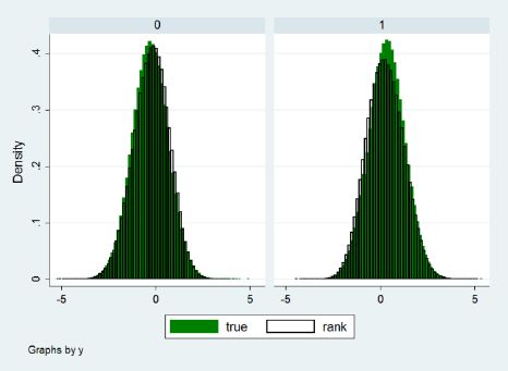
Finally, the Rank method is also able to replicate to a satisfactory extent the conditional distribution properties of the true individual effects. Figure 1, taken from Richiardi (2014), shows the distributions of the true and imputed individual effects for the y = 0 and y = 1 subsamples, in a Monte Carlo experiment where 1 million observations were drawn according to

Distribution of the true and imputed (via the Rank method) individual effects. Parameterization: x~N(−0.5,2),β = β = 1, α~N(0,1),η~N(0,1).
Source: Richiardi (2014).
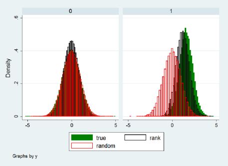
For extreme values of x, the Rank method introduces some distortions in the distribution of the individual effects, but still much lower than with random assignment (that is, sampling from the unconditional distribution of the individual effects). This can be seen in Figure 2, also taken from Richiardi (2014), for the first quintile of x.

Distribution of the true and imputed (via the Rank method) individual effects, first quintile of x. Parameterization: x~N(−0.5,2),β = β = 1, α~N(0,1),η~N(0,1).
Source: Richiardi (2014).
4. Female labor supply in Italy
The last decades have witnessed a long-term trend towards increasing female participation rates in most OECD countries. Nevertheless, there are persistent differences in levels suggesting that different countries are constrained by country-specific institutional and social factors. Ahn and Mira (2002) and Engelhardt et al. (2001) have divided the 21 OECD countries into three groups. The high participation group, in which the participation rate was, at the time of the study, above 60%, includes the U.S., Canada, the U.K., Sweden, Norway, Denmark, Finland and Switzerland. The medium participation group includes countries where the participation rate was in the 50–60% range. Finally, the low participation group includes Italy, Spain and Greece, where the female participation rate was lower than 50%. The latter group was also the target of the Lisbon 2000 Agenda, which set a goal of (at least) 60% for the female employment rate, to be achieved by 2010. By that year, the female employment rate in Italy was still close to 50%, followed only by Malta in the EU27 ranking.
Low female participation has always been a feature of the Italian labour market (Rondinelli & Zizza, 2011). Education matters in explaining the gender gap in participation rates: lower education levels are associated with larger gaps (Table 2). Even if participation rates of married women increased over the last several decades (Del Boca et al., 2006), employment rates of mothers with children under six in Italy are still very low (Del Boca, 2003): in facts, more than one fourth of women leave the labour market after a birth (Bratti et al. 2005; Casadio et al. 2008).
Participation rates by level of education, 2010.
| Italy | EU15 | |||
|---|---|---|---|---|
| Men | Women | Men | Women | |
| % | ||||
| Low education | 64.5 | 32.6 | 67.3 | 46.4 |
| Medium education | 80.7 | 63.1 | 82.2 | 71.2 |
| High education | 86.5 | 77.5 | 90.4 | 84.0 |
| TOTAL | 73.6 | 51.2 | 78.8 | 65.6 |
-
Source: our elaboration on Eurostat data
The following factors further help explaining the gender participation gap. First, in spite of the recent institutional changes, the Italian labour market still remains highly regulated: strict rules apply to hiring and firing and specify the types of available employment arrangements; these labour market regulations have been largely responsible for the high female and youth unemployment rates (Bertola et al., 2001). Thus, women have hard times to enter and re-enter (after breaks during childbearing years) the labour market. This situation affects also participation rates since discouraged women may decide to drop out of the labour force.
Second, part-time employment is still not common in Italy: it accounts for less than 30% of female employment, while it is above 75% in the Netherlands (Eurostat data for 2010): this is detrimental to the participation of married women, particularly those with children (Del Boca, 2002).
Third, women get a disproportionate share of the burden with respect to housework and child bearing within the family. In facts, the reconciliation of roles within and outside the family is more difficult for a working mother than for a working father, and often the strategies adopted are completely different: as the budget constraint becomes more binding men typically increase the time devoted to paid work and women decrease their working time or even exit the labour market (Anxo et al., 2007; Mencarini & Tanturri, 2004; Lo Conte & Prati, 2003).
Fourth, the public childcare system is inadequate and does not help enough in reducing the direct costs of participation; in particular, the number of available slots is limited with respect to OECD standards (especially in some regions in the South) and the hours of childcare offered are typically non compatible with full-time jobs. As for what concerns children in school age, things do not improve much as school days often end in the mid-afternoon, much earlier than the end of fulltime work days (Del Boca, 2002; Del Boca & Vuri, 2007).
Finally, a general cultural attitude against female participation in the labour market, which also partly explains the factors reviewed above, is only slowly fading away, as older generations are replaced by younger cohorts.
Of all these determinants, in our model we take explicitly into account the demographic evolution of the population and the changes in its composition by level of education, while we keep the institutional factors (labour market regulations and the public childcare system) as fixed. By considering a cohort effect, we proxy changes in the general cultural attitude, in the division of labour within the family and in the availability of part-time employment.
5. Data, econometric specifications and estimation results
5.1 The data
Estimations are performed on the Italian micro data from all eight waves 1994 to 2001 of the European Community Household Panel (ECHP).12 The ECHP was a survey conducted annually and provided detailed information on income, work and employment, poverty and social exclusion, housing, health, and many other diverse social indicators concerning living conditions of private households and individuals (aged 16+). Cross section and longitudinal weights were provided in order to achieve representativeness of the total population. The main advantage of ECHP is that it allows analysing participation in the labour market, schooling and household formation from a dynamic point of view.
The initial population is a random extraction (with replacement) from the 2001 Italian subsample of the ECHP. A large part of the initial population is therefore included in the estimation sample, a case which would make it possible to use the estimated individual effects, rather than imputing them. As we will explain in the validation section, we exploit this continuity between the estimation sample and the simulation sample to assess the advantages of the Rank method over the simpler solutions of imputing a null individual effect or sampling from the unconditional distribution of the individual effects.
Notwithstanding some disruptions in the time series of indicators between the ECHP and the EU-SILC data due to changes in the sampling strategy, in the structure of the questionnaire and in some of the definitions (European Communities, 2005), we use the 2005–2008 Italian data of the EU-SILC to perform validation analysis of the different simulation approaches.13
5.2 Modelling approach
In the econometric literature, there are two ways of treating UH: random effects or fixed effects models. Interested readers can refer to Honoré (2002) for a full discussion on the choice between these two approaches. This paper follows the random effects approach in order to have a fully specified model in which one can estimate all the quantities of interest, including the coefficients of time invariant characteristics (e.g. gender). This allows not only to interpret the coefficients correctly –as in standard microeconometric papers–burden of different but, of most importance here, to simulate forward the evolution of the initial population. The random effects approach usually lead to more efficient estimators of the parameters of the model if the distributional assumptions are satisfied. Moreover, traditional maximum likelihood estimator of non-linear panel data models with fixed effects generally exhibits considerable bias in finite sample when the number of periods is not large.14
In order for the model to be fully parameterized, initial conditions have to be specified. An initial condition problem arises when the start of the observation period does not coincide with the start of the stochastic process generating individual experiences (Heckman, 1981a; Arulampalam et al., 2000).15 Our way to deal with this issue is to use the estimator suggested by Heckman (1981a, 1981b). His approach involves the specification of an approximation to the reduced form equation for the initial condition and allows for cross-correlation between the dynamic equation and the initial condition:
where zi,0 is a vector of exogenous covariates (including xi,0 and, eventually, additional variables that can be viewed as “instruments” such as pre-sample variables).16 Exogeneity corresponds to θ = 0 and can be tested accordingly. Equations (3), (4) and (6) together specify a complete model for the process that can be estimated by maximum likelihood (for details about the estimation see Arulampalam and Steward, 2007).
We use a random effects dynamic probit model for estimating male and female labour force participation, unemployment and living in consensual union. For these processes, we also estimate simple probit models. The other processes (education and fertility) are also modelled by means of probit models.
5.3 Initial status
ECHP and EU-SILC data cover individuals aged 16+. Since we need information on lagged status, individuals enter the simulation at age 17. Assignment to the initial status (in education, activity, employment) is random, based on observed probabilities (Table 3).
Status at age 17.
| In education | Active Males | Unemployed | |
|---|---|---|---|
| North | 79.8% | 17.2% | 8.6% |
| Centre | 86.0% | 10.4% | 15.0% |
| South | 82.3% | 12.2% Females | 46.9% |
| North | 86.7% | 12.1% | 19.0% |
| Centre | 86.8% | 10.2% | 35.0% |
| South | 83.7% | 9.9% | 55.8% |
-
Source: our elaboration on Italian LFS data (2001).
As a scenario, we assume that the share of individuals aged 17 who are in education will (linearly) converge to 100% from the initial level in Table 3 by the end of the simulation period (2050).
5.4 Education
In Italy school attendance is compulsory until age 16, while it is generally illegal to work under 15.17 Primary school has 8 grades, and students should normally complete it at 13–14. Then, they compulsorily enrol in secondary school, which should last for 5 years. According to Sistan (2006, 2007), secondary school attendance from age 16 to age 18 is above 80% (2005 data), while the probability of achieving a diploma is slightly above 70% (67% for males and 78% for females). Early school leavers (individuals aged 18–24 that achieved at least an education level equal to ISCED 2) are about 22%, higher than the EU-25 average (15%).
Among those who achieved a diploma, three in four enrol at university (79% females; 66% males); overall, university enrolment rate is about 56%, about the OCSE average (54%). Enrolment rates have increased from 1998 to 2005 (+16%). Dropouts after the first year of university are about 20%, and they remain significant even later. Less than one in two students enrolled actually graduate (51% females; 37% males). Among those who make it, 52% graduates before age 25 and 80% before age 29. Graduation rates have remained fairly stable over the years. Very few people come back to formal education, once left.
Coherently with this picture, we estimate two separate equations, one for secondary school attendance and one for university attendance.18 In both cases the probability of being a student at time t is modelled as a function of sex, age, age-squared, year of birth and area of residence, and estimation is conditioned on not having entered the labour market. Estimates are reported in Table 4. The probability of being enrolled in secondary school decreases with age, as individuals are supposed to take a diploma at about 18–19 years old.
Enrolment.
| Secondary School (Probit) | University (Probit) | |||||
|---|---|---|---|---|---|---|
| Coef | SE | Coef. | SE | |||
| Female | −0.008 | 0.069 | 0.113 | * | 0.055 | |
| Age | −11.285 | ** | 2.665 | 0.691 | ** | 0.214 |
| Age-squared | 0.287 | ** | 0.070 | −0.016 | ** | 0.004 |
| Centre | 0.090 | 0.098 | 0.010 | 0.070 | ||
| South | 0.087 | 0.081 | 0.110 | ** | 0.033 | |
| Year of birth | 0.073 | ** | 0.021 | 0.036 | ** | 0.014 |
| Constant | −33.024 | 50.76 | −77.856 | ** | 27.901 | |
-
Source: our elaboration on ECHP 1994–2001 data.
-
*
significant at 90% confidence level.
-
**
significant at 95% confidence level.
-
*** significant at 99% confidence level
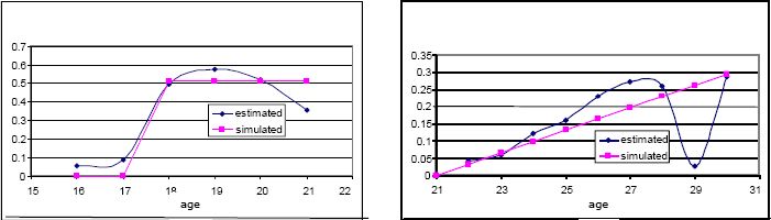
Unfortunately, the exact moment of graduation is often only poorly observed in ECHP. For this reason, in the microsimulation we use the same coefficients for graduation as in Leombruni and Richiardi (2006), estimated on the 1993–2003 Italian Labor Force Surveys (RTFL) data. Graduation is modelled by means of a constant probability in the relevant age brackets for secondary school, and with a linear term in age for university (Figure 3).

Probability of graduating, high school (left panel) and university (right panel).
Source: Leombruni and Richiardi (2006).
5.5 Unemployment and male participation
The unemployment status at time t is modelled as function of lagged unemployment status, age, education level, area of residence, the status of student at time t-1 and the overall unemployment rate.
Male participation at time t is modelled as a function of lagged participation, age, year of birth, education level, area of residence and student status at time t-1. In both cases, model estimation is conditioned on not being retired or student. We first estimate standard probit models. To account for UH and solve the initial conditions problem, we then estimate dynamic random effects models. The estimated coefficients and standard errors are shown in Table 5. To compare the probit coefficients with those from the random effects estimators, the latter need to be multiplied by an estimate of 1/√(1+σα2), where σα represents the size of UH (see Arulampalam, 1999). Allowing for the different normalizations, the scaled estimate for lagged participation (unemployment) is 0.54 (0.70), significantly less than the pooled probit estimate. Participation (unemployment) yesterday increases the probability of participating (being unemployed) today. The relationship between male participation and age follows the usual inverse U-shape. Higher education increases male participation and decreases the probability of being unemployed. Living in the south of Italy decreases male participation and increases the probability of being unemployed.
Unemployment and male participation estimates (Table legend).
| Unemployment | Male participation | |||||||
|---|---|---|---|---|---|---|---|---|
| Probit | Dynamic RE model | Probit | Dynamic RE model | |||||
| Coef. | Robust SE | Coef. | SE | Coef. | Robust SE | Coef. | SE | |
| Lag (participation) | --- | --- | --- | --- | 1.766 ** | 0.052 | 0.799 ** | 0.077 |
| Lag (unemployment) | 1.785 ** | 0.026 | 1.123 ** | 0.039 | --- | --- | --- | --- |
| Female | 0.356 ** | 0.022 | 0.592 ** | 0.049 | --- | --- | --- | --- |
| Age | −0.148 ** | 0.009 | −0.256 ** | 0.020 | 0.130 ** | 0.011 | 0.326 ** | 0.026 |
| Age^2 | 0.002 ** | 0.0001 | 0.002 ** | 0.000 | −0.002 ** | 0.000 | −0.004 ** | 0.000 |
| High education | −0.246 ** | 0.038 | −0.582 ** | 0.083 | 0.287 ** | 0.066 | 0.341 ** | 0.115 |
| Medium education | −0.237 ** | 0.022 | −0.368 ** | 0.045 | 0.110 ** | 0.032 | 0.170 ** | 0.058 |
| Centre | 0.283 ** | 0.035 | 0.463 ** | 0.078 | −0.054 | 0.046 | −0.104 | 0.088 |
| South | 0.783 ** | 0.028 | 1.508 ** | 0.065 | −0.155 ** | 0.035 | −0.313 ** | 0.069 |
| Year of birth | --- | --- | --- | --- | −0.006 | 0.007 | 0.010 | 0.014 |
| Lag (student) | 1.147 ** | 0.043 | 0.504 ** | 0.116 | 0.205 ** | 0.061 | −0.026 | 0.135 |
| Unempl.rate | 11.354 ** | 1.585 | 10.076 ** | 2.828 | --- | --- | --- | --- |
| _cons | −0.167 | 0.229 | 1.403 ** | 0.476 | 9.376 | 13.075 | −24.420 | 27.245 |
| σα | --- | 1.256 | --- | 1.071 | ||||
-
Source: our elaboration on ECHP 1994–2001 data.
-
*
significant at 90% confidence level.
-
**
significant at 95% confidence level.
-
***
significant at 99% confidence level.
5.6 Female labour market participation and household formation
We estimate two separate equations, one for labour market participation and one for the choice of living in consensual union.19 Reflecting our interest in uncovering the presence of dynamic spillover effects from participation to marriage, and from marriage to participation, the equations for female labour market participation and household formation also include cross-effect lagged variables, which are assumed weakly exogenous. Therefore, both participation and living in consensual union at time t are modelled as a function of lagged participation, lagged consensual union status, the existence of children under three (at time t-1), age, year of birth, level of education, area of residence and being a student (at time t-1). Moreover, model estimation is conditioned on not being retired or a student at time t. Dummies for the area of residence also capture regional differences in the availability of childcare and other (local) institutional factors. In order to simplify the model and keep a dichotomous participation outcome variable we do not explicitly model work hours. This implies that we do not consider the availability of part-time. Since the share of female part-time employment in the total employment has increased almost linearly since 1990, from about 10% to about 30% with few regional differences, this increase is captured by the cohort effect.20
As a benchmark, the estimates of the standard pooled probit models are reported in Table 6, columns 1 and 2. Then, column 3 and 4 report the coefficients and standard errors of the dynamic probit model with random effects. As explained above, the random effects probit and pooled probit models involve different normalizations. The scaled estimate of the coefficient on lagged participation (living in consensual union) is 0.90 (2.25), significantly less than the pooled probit estimate: this indicates that omitting permanent UH leads to overestimation of state dependence. There is a lot of heterogeneity that cannot be accounted for by the explanatory variables: the estimated σα is equal to 1.2 (0.89). Instead, the estimated coefficients on the other covariate are similar (sometime larger) than the pooled estimates.
Female participation and household formation estimates.
| Female participation | Living in consensual union | |||||||
|---|---|---|---|---|---|---|---|---|
| Probit | Dynamic RE model | Probit | Dynamic RE model | |||||
| Coef. | Robust SE | Coef. | SE | Coef. | Robust SE | Coef. | SE | |
| Lag (participation) | 2.387 ** | 0.027 | 1.417 ** | 0.038 | −0.049 | 0.033 | −0.093 | 0.052 |
| Lag (union) | −0.417 ** | 0.027 | −0.595 ** | 0.049 | 3.795 ** | 0.043 | 3.010 ** | 0.075 |
| Lag (children under 3) | −0.159 ** | 0.032 | −0.197 ** | 0.050 | 0.347 ** | 0.098 | 0.516 ** | 0.122 |
| Age | 0.038 ** | 0.007 | 0.087 ** | 0.015 | 0.074 ** | 0.010 | 0.263 ** | 0.036 |
| Age2 | −0.001 ** | 0.000 | −0.001 ** | 0.000 | −0.001 ** | 0.000 | −0.003 ** | 0.000 |
| High education | 0.808 ** | 0.047 | 1.665 ** | 0.093 | −0.001 | 0.060 | −0.170 | 0.093 |
| Medium education | 0.371 ** | 0.021 | 0.775 ** | 0.044 | −0.029 | 0.032 | −0.135 * | 0.057 |
| Centre | −0.116 ** | 0.027 | −0.355 ** | 0.064 | 0.052 | 0.042 | 0.145 * | 0.073 |
| South | −0.270 ** | 0.021 | −0.738 ** | 0.052 | 0.015 | 0.031 | 0.003 | 0.053 |
| Year of birth | 0.000 | 0.004 | 0.009 | 0.008 | 0.002 | 0.007 | −0.026 | 0.014 |
| Lag(student) | 0.549 | 0.056 | 0.272 * | 0.121 | −0.530 ** | 0.066 | −0.706 ** | 0.090 |
| _cons | −1.326 | 7.845 | −19.025 | 16.684 | −7.667 | 13.146 | 44.404 | 28.285 |
| σα | ---- | 1.218 | ---- | 0.890 | ||||
-
Source: our elaboration on ECHP 1994–2001 data.
-
*
significant at 90% confidence level.
-
**
significant at 95% confidence level.
-
***
significant at 99% confidence level.
Estimated coefficients generally have the expected sign: participation at time t-1 increases the probability of participating at time t, while living in consensual union and having small children reduce it; having a better education is associated with higher activity rates, while living in the Centre and especially in the South of Italy is associated with lower activity rates.
Quite obviously, we find that living in consensual union in any one year strongly increases the probability of living in consensual union in the next year. The probability also increases if the woman has young children. The relationship with age is again inverse U-shaped. The level of education and the area of residence are not significant; instead, being a student at time t-1 reduces the probability of living in consensual union at time t.
Finally, we estimate the probability of having a child at time t, as a function of the presence of children aged under three at time t-1, the number of children at time t-1, dummies about the labour market status at time t-1 (in education, in the labour force, in employment), age, level of education, area of residence and the overall fertility rate. Estimation is conditioned on living in consensual union and being in the age bracket 17–45. Estimates are reported in Table 7. Again, the coefficients go in the expected direction: the probability of having a child later initially increases and then decreases with age, decreases if in the household there are already children under three, decreases with the number of children in the household. Having high education increases the probability of having a child, for a given age. No significant geographical differences are found.
Birth probability estimates the sample includes only women aged 17–45.
| Motherhood | Probit | |
|---|---|---|
| Coef. | Robust SE | |
| Lag (children under 3) | −0.571 ** | 0.050 |
| Lag (no children) | −0.371 ** | 0.084 |
| Lag (participation) | −0.037 | 0.046 |
| Lag (unemployment) | −0.087 | 0.072 |
| Lag (student) | −0.216 | 0.153 |
| Age | 0.287 ** | 0.043 |
| Age2 | −0.006 ** | 0.001 |
| High education | 0.227 ** | 0.072 |
| Medium education | 0.039 | 0.043 |
| Centre | 0.062 | 0.060 |
| South | 0.092 | 0.073 |
| Fertility rate | 11.716 * | 5.106 |
| Constant | −4.628 ** | 0.722 |
-
Source: our elaboration on ECHP 1994–2001 data.
-
*
significant at 90% confidence level.
-
**
significant at 95% confidence level.
-
***
significant at 99% confidence level.
6. The microsimulation model
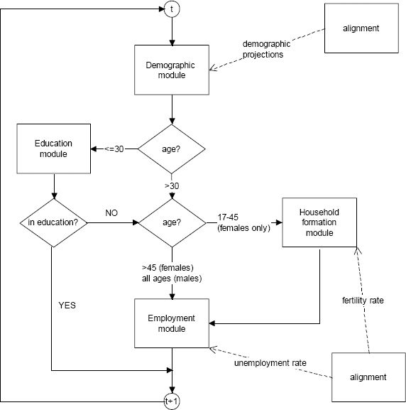
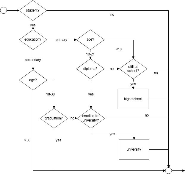
Our model is a discrete-time dynamic microsimulation of labour supply, with an open population: flags are switched on and off for partners and children for the female population, but no simulated individuals are actually matched. The microsimulation is comprised of four modules: Demography, Education, Household formation and Employment. Individuals are simulated in the age bracket 17–54, from 2002 to 2050. The overall structure of the microsimulation is depicted in Figure 4. Standard simulation runs involve a base year population of about 40,000 individuals, representative of 60 million Italians.

Structure of the microsimulation model.
6.1 Demographic module
Population is aligned to official demographic projections by year, age, gender and macro-area of living (North, Centre and South of Italy). Whenever the population is over-represented in a given age, gender and area cell, simulated individuals are killed at random. Whenever the population is under-represented, new individuals are created by cloning at random existing individuals in the same cell (in adjacent cells if the cell is empty). We do not model (internal nor external) migration.
6.2 Education module
We separately model enrolment and graduation, both for secondary school and university. Individuals enter the simulation at 17, after completion of compulsory education. Dropouts at 16 are modelled by aligning the initial status (in education, in the labour force, in employment) to the observed frequencies (see Table 3 above). Dropouts from school exit the education module and enter the labour market module. Students can graduate from secondary school starting at age 18. Those who fail to graduate before age 22 exit the education module and enter the labour market module. Secondary school graduates can enter university. University participation is allowed until age 30, while graduation can take place beginning at age 21. University dropouts leave the education module and enter the labour market module. We make the simplifying assumption that people never go back to education, once they have left. This is justified, as already discussed, by the very small number of students of older ages.
The detected (linear) trends toward higher high school participation are stopped for individuals born in 1990 or later, while those toward higher university participation are stopped for individuals born in 1985 or later (we prudentially assume all trends have already come to an end in the base year).
The flowchart of the Education module is represented in Figure 5.

The education module.
6.3 Household formation module
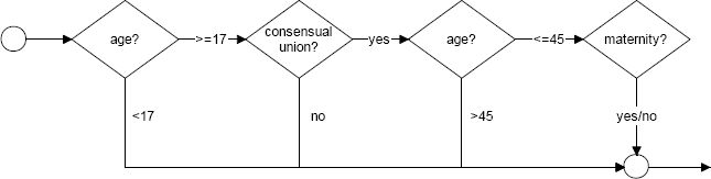
Given that the presence of a partner is not relevant, at a first order approximation, for male labour market participation, the household formation module is only applied to the female population.21 The module is comprised of two sub-modules: Living in consensual union and Maternity. Women aged 17 or older and who are not student can enter a consensual union. Note that at young ages not living in consensual union is likely to be a choice, while at older ages it might also reflect a partner’s death, hence a state of widowhood. The (linear) cohort effect in the equation for living in consensual union is stopped for individuals born in 1990 or later. Women aged 17–45 who live in a consensual union can have children. The total amount of births in each year is aligned with demographic data. The flowchart of the Household formation module is represented in Figure 6.

The Household formation module (females only).
6.4 Employment module
The labour market module is applied to all individuals who are not in education or retired (remember individuals enter the simulation above the minimum working age). We consider retirement only for those individuals who are already retired in the initial population, and assume no one can retire before age 55 as the simulation proceeds (this is in line with the recent reforms of the Italian pension system).
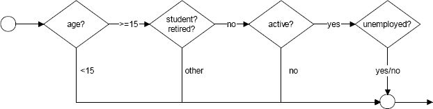
The employment module is composed of two sub-modules: Labour market participation and Unemployment. Labour market participation is modelled separately by gender, and the model for females is conditional on household composition. The (linear) cohort effects in the equations for labour market participation are stopped for individuals born in 1990 or later. Alignment with an exogenous trend is performed for the overall unemployment rate for the 17–54 population. Consequently, the Unemployment module is to be regarded as a model of unemployment rate differentials, rather than unemployment rate levels. This is justified by the fact that we do not model the demand side: the overall unemployment rate is therefore considered as an exogenous parameter of the simulation. The flowchart of the Employment module is represented in Figure 7.
The employment module.
7. Model comparison and validation
The credibility of a dynamic microsimulation model is based on its capacity to reproduce observed data or known benchmarks such as outside projections. Accordingly, an important aspect of dynamic microsimulation modelling is the validation of results produced by the simulation exercise. However, the applied literature has devoted little attention to validation procedures and the quantification of uncertainty around model predictions (Wolf, 2001), and there is currently no apparent consensus among practitioners on what constitutes a best practice. In this section, we focus on a specific aspect of validation: ex-post validation of model outcome. With the limitations arising from the fact that the ECHP was discontinued in 2001 and replaced only in 2004 by a different survey (EU-SILC), and the fact that the most recent years cannot be used for validation due to the impact of the Great Recession, we compare the simulated female participation rates with the actual participation trends computed on the Italian EU-SILC data over the period 2005–2008.22 The four versions of the model that we test are labelled Probit (pooled probit estimates), Null (dynamic random effect probit estimates without imputation of random effects), Unconditional (dynamic random effect probit estimates with imputation of random effects from the unconditional distributions), Rank (dynamic random effect probit estimates with imputation of random effects by means of the Rank method).
Figure 8 shows the projected activity rates in the age group 17–54. Depending on the estimation method we get significant differences in both males and females participation rates. For females, these differences become larger over time: at the end of the simulation period, the difference between predictions obtained under the Rank and the Null scenario amounts to almost 10 percentage points. This corresponds almost exactly to the bias we expect due to nonlinearity of the probit transformation, for the estimated standard deviation of the individual effects: +4% (+8%) for the Null scenario at the beginning (end) of the simulation period, when the average activity rate under the Rank scenario is .57 (.65). Also expected, given the theoretical results (Richiardi, 2014), is the similarity between the Rank and the Unconditional scenario, when cross-sectional figures are considered.
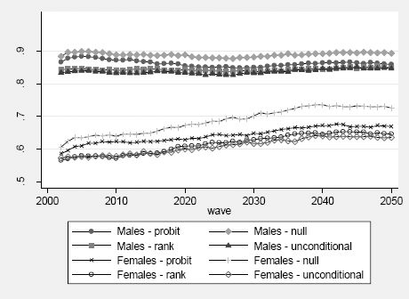
Projected participation rates, individuals aged 17–54.
The simulation projections can be compared with the observed participation rates for the period 2005–2008 as computed using EU-SILC data (Table 8). Predictions obtained using the Rank method and those obtained sampling from the unconditional distributions of the individual effects are slightly lower than the observed activity rates both in term of average and transition probabilities. The true data lie in between the Probit and the Rank/Unconditional forecasts. The Null forecasts do indeed overestimate both female participation rates and transition probabilities in and out the labour market. Hence, improving the estimates of the coefficients by considering UH but failing to impute it to the simulated population results in forecasts that are even worse than forecasts based on simpler (and misspecified) models.
Validation results: female participation rates (%), individuals aged 17–54.
| True data | Simulated data | |||||
|---|---|---|---|---|---|---|
| Dataset | Probit | Null | Rank | Unconditional | ||
| ECHP | 1994 | 52.85 | ||||
| 1995 | 53.22 | |||||
| 1996 | 53.66 | |||||
| 1997 | 53.80 | |||||
| 1998 | 55.52 | |||||
| 1999 | 55.49 | |||||
| 2000 | 54.76 | |||||
| 2001 | 56.24 | |||||
| EUSIC | 2005 | 59.78 | 61.02 | 63.41 | 58.01 | 57.48 |
| 2006 | 60.28 | 61.77 | 63.83 | 57.91 | 57.89 | |
| 2007 | 59.10 | 61.77 | 64.26 | 57.81 | 58.01 | |
| 2008 | 60.07 | 62.34 | 64.06 | 57.78 | 57.93 | |
| Probability of participate at time t | ||||||
| if not participate at t-1 | 17.06 | 14.22 | 34.69 | 20.29 | 20.68 | |
| if participate at t-1 | 91.05 | 93.79 | 85.78 | 89.09 | 88.41 | |
| Probability of not participate at time t | ||||||
| if not participate at t-1 | 82.94 | 85.78 | 65.31 | 79.71 | 79.32 | |
| if participate at t-1 | 8.5 | 6.21 | 14.22 | 10.91 | 11.59 | |
The practical equivalence between imputing individual effects via the Rank method or sampling from the unconditional distributions breaks down dramatically when individual life histories are considered.
To document this, we have estimated the same simple probit models as described in Section 5 on couples of adjacent years: the first set of estimates is performed on 2000–2001, entirely on ECHP data; the second set is performed on 2001–2002, by merging the first year of the simulation output with ECHP data; then, other sets follow entirely on simulation data.23 We are interested in the coefficient of the lagged endogenous variable, as a descriptive measure of state persistence. Table 9 shows the results.24 The first column refers to the years 2000–2001 and is computed on true data: it is thus invariant to the model considered and constitutes our target. The second column is computed using the true data as base year (2001) and the first period of the simulated data as final year (2002): it thus encompass any discontinuity in life trajectories due to the imputation method. Theory suggests that state persistence (the coefficients of the lagged endogenous variables) should be lower for the Unconditional scenario, intermediate for the Null scenario and higher (though still below the target) for the Rank scenario. The third column reports the averages of the coefficients of the lagged endogenous variables computed over the couples of years 2002–2003 to 2007–2008, estimated on simulated data. Theory now suggests that state persistence should pick up again, with the coefficients under the Rank and the Unconditional scenario broadly similar and higher than those under the Null scenario. This is broadly in line with what we find. State persistence decreases in the first year of the simulation for the Unconditional scenario, as the true individual effects governing past outcomes are replaced by random draws from the unconditional distributions, which are by definition uncorrelated with the true individual effects. From the second year of the simulation onward state persistence picks up again, and individual trajectories keep the memory of the artificial discontinuity of the previous year. Under the Null scenario, on the other hand, state persistence decreases less that under the Unconditional scenario on the first year, but then remains stationary at this level. Only under the Rank scenario state persistence remains reasonably close to the true value, keeping the discontinuity of lifetime trajectories in the first period of the simulation at a minimum.
Coefficients of lagged endogenous variables (standard errors in parenthesis), same probit models as for input estimation. Estimation is performed on couple of years (the third column reports averages over results from 2002–2003 to 2007–2008).
| ECHP | ECHP/sim | sim | |
|---|---|---|---|
| 2000–2001 | 2001–2002 | 2002–2008 | |
| Union unconditional | 3.810 (0.087) | 1.648 (0.019) | 2.626 (0.034) |
| Null | 3.810 (0.087) | 2.285 (0.022) | 2.150 (0.036) |
| Rank | 3.810 (0.087) | 3.111 (0.026) | 2.826 (0.035) |
| Participation (males) unconditional | 2.550 (0.075) | 1.426 (0.024) | 1.728 (0.033) |
| Null | 2.550 (0.075) | 1.901 (0.026) | 1.763 (0.051) |
| Rank | 2.550 (0.075) | 2.599 (0.028) | 1.858 (0.308) |
| Participation (females) unconditional | 2.542 (0.056) | 0.638 (0.015) | 1.856 (0.024) |
| Null | 2.542 (0.056) | 0.974 (0.015) | 0.938 (0.024) |
| Rank | 2.542 (0.056) | 2.057 (0.017) | 1.990 (0.024) |
8. Conclusions
In this paper we have dealt with the problem of assigning unobserved individual effects to the simulation sample, when new individuals enter the simulation with a history of previous outcomes. The only theoretically sound methodology in this case is sampling from the estimated conditional distributions, which can be fairly complicated in nonlinear models. Using a dynamic microsimulation model of labour supply in Italy as a testbed, we have shown that neglecting the problem (i.e. assigning a null effect to all individuals) implies a forecasting bias in discrete choice models, due to nonlinearity of the probit/logit transformations. Sampling from the unconditional estimated distributions of the individual effects prevent the forecasting bias, hence getting cross-sectional statistics right, but introduces unnatural breaks in individual trajectories at the moment of imputation, therefore getting longitudinal statistics wrong. The same applies if the estimates are obtained under simple specifications without unobserved heterogeneity. We have then provided a first empirical application of a new algorithm that greatly reduces the complexity of sampling from the conditional distributions, at the cost of introducing a small correlation between the imputed individual effects and the individual observable characteristics. Our results have been validated on out-of sample data, albeit admittedly short. Imputing individual effects with the new method allows to remain more on track with observed data both cross-sectionally and longitudinally.
Finally, from a substantive point of view, our microsimulation documents the existence of a marked though slow process of convergence in the activity rates of different subgroups of the Italian population: between men and women, between women with children and women without children, between the North and the South of Italy.
Footnotes
1.
He also develops an optimal assignment algorithm for the binary response model, which works in quadratic time rather than in third or fourth order polynomial time as the standard algorithms.
2.
The same argument applies, mutatis mutandis, to a multinomial setting with more than two states.
3.
An alternative approach is to use Markovian transitions models, where the processes are split up according to the initial state. This amounts to estimate
or, equivalently,
The main advantage of this approach is the possibility to allow estimated persistence to vary according with the initial state and the observed individual characteristics, at the cost of a higher number of parameters.
4.
In facts, we can get significant estimates of state dependence coefficients even when there is no true state dependence and persistence is only due to permanent UH (Carro, 2007).
5.
See also Cramer (2005).
6.
For applications to models of labour supply, see for instance Haan (2006) and Pacifico (2009).
7.
Richiardi (2014) also discusses a fourth option of imputing the missing variables in the simulation sample from their estimated counterparts in the estimation sample. This solution however turns out to be suboptimal and feasible only in special cases.
8.
See Gu et al. (2009) for an application to a random effects binary probit model with heteroscedasticity.
9.
A proper survey of the treatment of UH in dynamic microsimulation models is hampered by the fact that the relevant papers generally devote little space to the presentation of the econometric estimates –sometimes even the list of covariates is missing. This is a well-known problem with the microsimulation approach: being in general large models, developed over the course of many years and often building on pre-existing work, microsimulation models end up being close to black boxes. Sometimes detailed explanations can be found in technical papers that however remain unpublished or have a limited circulation, while published articles often restrict their attention, given the page constraint, on some specific result or addition to the basic model.
10.
See Richiardi (2014) for more details.
11.
Indeed, an improper treatment of UH might contribute to explain why alignment becomes necessary.
12.
The ECHP was discontinued in 2001 and replaced only three years later by the European Union Statistics on Income and Living conditions (EU-SILC).
13.
The Italian component of the EU-SILC panel data is available only from 2005 onwards.
14.
Fixed effects estimators of nonlinear panel model can be severely biased due to the incidental parameters problem. This problem arises because unobserved individual characteristics are replaced by sample estimates, biasing estimates of model parameters. As far as we know, the solution proposed are not sqrt(N)-consistent (Honoré and Kyriazidou, 2000; Hahn, 2001; Honoré and Tamer, 2004). Some authors propose modified maximum likelihood estimators that reduces the order of the bias (i.e. Cox and Reid, 1987; Arellano, 2003; Carro, 2007; Arellano and Hahn, 2007; Val, 2009). The latter estimators work only “moderately” well when the number of periods T is larger than 8, but this is not our case. Recently, Hoderlein et al. (2011) has proposed a nonparametric procedure that generalizes the conditional logit approach leading to an estimator based on nonlinear stochastic integral equations that seems to works moderately well in finite sample Monte Carlo simulations. Also, the random effect model can be generalized to allow for some correlation between the individual effects and the regressors. Following the Mundlak-Chamberlain approach (Mundlak, 1978; Chamberlain, 1982), this reduces to running a random-effect model where the individual means of the time-varying characteristics are added as control variables to allow for some correlation with the random effects.
15.
In dynamic panel data models with unobserved effects, the initial condition problem is an important issue. Many authors studied dynamic linear models with an additive unobserved effect with a special focus on the treatment of the initial condition problem (see, for example, Ahn and Schmidt, 1995; Anderson and Hsiao, 1982; Arellano and Bond, 1991; Arellano and Bover, 1995; Blundell and Bond, 1998; Hahn, 1999]). The initial condition problem is much more difficult to resolve within non-linear models. Honoré (1993) and Honoré and Kyriazidou (2000) offer examples of the treatment of the initial condition problem in a semi-parametric context. The interested reader can also refer to Heckman (1981a, 1981b), Hsiao (1986), Orme (1997) and Wooldridge (2005b) for a discussion of alternative ways of handling initial conditions in a dynamic non-linear model with UH, which however provide similar results (Arulampalam & Stewart, 2007). The Mundlak-Chamberlain approach for dealing with correlated random effects can also be applied to these estimators.
16.
If the vector zi does not include instruments, the model is identified by the functional form.
17.
Illegal dropouts are approximately zero in primary school and about 1.5% in secondary school (Sistan, 2006).
18.
Dario Di Pierro helped with the estimates.
19.
Female labour force participation and the choice of living in consensual union may of course be correlated. A joint determination of female participation and marital status can be treated extending the dynamic random effects model allowing for correlation in the error terms (see Alessie et al., 2004; Devicienti and Poggi, 2011). Since this is not the focus of the present paper, we do not consider this issue further.
20.
In 2010 the share of female part-time employment was 30.5% in the North, 29.0% in the Centre and 25.4% in the South (Italian LFS data).
21.
Living in union might well affect the decision about how much to work, and possibly wages; however, we do not model work hours, nor wages.
22.
A presentation of the long-term projections that come out of the model is contained in the working paper version of our work (Richiardi & Poggi, 2012).
23.
This validation strategy exploits the fact that the initial population in the simulation coincides with the last sample used for estimation. This, together with our desire to use all years from 2005 to 2008 for validation, explains why we have used a 2001 sample from ECHP data rather than a 2005 sample from EU-SILC data for our initial population.
24.
We do not report results for unemployment as this process is subject to alignment.
References
-
1
Labor Supply Responses and Welfare Effects of Tax ReformsScandinavian Journal of Economics 97:635–659.
-
2
Efficient estimation of models for dynamic panel dataJournal of Econometrics 68:5–28.
-
3
Models for Retirement Policy Analysis. Report prepared for the Society of ActuariesModels for Retirement Policy Analysis. Report prepared for the Society of Actuaries.
-
4
Formulation and estimation of dynamic models using panel dataJournal of Econometrics 68:5–27.
-
5
Time Allocation between Work and Family Over the Life-Cycle: A Comparative Gender Analysis of Italy, France, Sweden and the United States. IZA Discussion Paper. No. 3193Time Allocation between Work and Family Over the Life-Cycle: A Comparative Gender Analysis of Italy, France, Sweden and the United States. IZA Discussion Paper. No. 3193, November.
- 6
-
7
Some tests of specification for panel data: Monte Carlo evidence and an application to employment equationsReview of Economic Studies 58:277–297.
-
8
Another look at the instrumental variables estimation of error component modelsJournal of Econometrics 68:29–51.
-
9
Understading bias in nonlinear panel models: Some recent developments, 3R Blundell, WK Newey, T Persson, editors. Cambridge: Cambridge University Press.
-
10
A Note on estimated effects in random effect probit modelsOxford Bulletin of Economics and Statistics 61:597–602.
-
11
Simplified Implementation of the Heckman Estimator of the Dynamic Probit Model and a Comparison with Alternative Estimators”. IZA discussion paperSimplified Implementation of the Heckman Estimator of the Dynamic Probit Model and a Comparison with Alternative Estimators”. IZA discussion paper, No. 3039, Institute for the Study of Labor, Bonn.
-
12
Unemployment persistence. Oxford Economic Papers24–50, Unemployment persistence. Oxford Economic Papers, 52.
-
13
Welfare and Employment in a United EuropeWelfare Systems and Labor Markets in Europe: what convergence before and after EMU?”, Welfare and Employment in a United Europe, MIT Press, Cambridge, MA.
-
14
Initial conditions and moment restrictions in dynamic panel data modelsJournal of Econometrics 87:115–143.
-
15
New mothers’ labour force participation in Italy: The role of job characteristicsLabour 19:79–121.
-
16
Assignment Problems - Revised ReprintPhiladelphia: Society for Industrial and Applied Mathematics.
-
17
Algorithms and Codes for the Assignment ProblemAnnals of Operations Research 13:193–223.
-
18
Estimating dynamic panel data discrete choice models with fixed effectsJournal of Econometrics 140:503–528.
-
19
Balancing work and family in Italy: New mothers’ employment decisions after childbirth. Bank of Italy Economic working papers684, Balancing work and family in Italy: New mothers’ employment decisions after childbirth. Bank of Italy Economic working papers, Temi di discussione.
- 20
-
21
Parameter orthogonality and approximate conditional inferenceJournal of the Royal Statistical Society 49:1–39.
-
22
Omitted Variables and Misspecified Disturbances in the Logit Model. Tinbergen Institute Discussion Paper. TI 2005-084/4Omitted Variables and Misspecified Disturbances in the Logit Model. Tinbergen Institute Discussion Paper. TI 2005-084/4.
-
23
Discrete hours labour supply modelling: specification, estimation and simulationJournal of Economic Surveys 19:697–734.
-
24
The effect of child care and part time opportunities on participation and fertility decisions in ItalyJournal of Population Economics 15:1432–1475.
-
25
Why are fertility and participation rates so low in Italy (and Southern Europe)?Paper prepared for presentation at the Italian Academy at Columbia University.
-
26
Labour market participation of women and fertility: the effect of social policiesMimeo: University of Turin.
-
27
The mismatch between employment and child care in Italy: the impact of rationingJournal of Population Economics 20:805–832.
-
28
Poverty and social exclusion: two sides of the same coin or dynamically interrelated processes?Applied Economics 43:3549–3571.
-
29
The continuity of indicators during the transition between ECHP and EU-SILCLuxembourg: Office for Official Publications of the European Communities.
-
30
Household Demography and Household ModelingCompeting Risks and Unobserved Heterogeneity with Special Reference to Dynamic Microsimulation Models, Household Demography and Household Modeling, Springer-Verlag, New York, NY.
- 31
-
32
Bayesian estimation of a random effects heteroscedastic probit modelThe Econometrics Journal 12:324–339.
-
33
Slowly, But Changing: How Does Genuine State Dependency Affect Female Labor Supply On The Extensive and Intensive Margin. JEPS Working Papers. No. 06-002, JEPSSlowly, But Changing: How Does Genuine State Dependency Affect Female Labor Supply On The Extensive and Intensive Margin. JEPS Working Papers. No. 06-002, JEPS.
-
34
The information bound of a dynamic panel logit model with fixed effectsEconometric Theory 17:913–932.
-
35
How informative is the initial condition in the dynamic panel data model with fixed effects?Journal of Econometrics 93:309–326.
-
36
Studies in Labor MarketsHeterogeneity and state dependence”, Studies in Labor Markets, Chicago Press, Chicago, IL.
-
37
The incidental parameters problem and the problem of initial conditions in estimating a discrete time-discrete data stochastic process”In: CF Manski, D McFadden, editors. Structural Analysis of Discrete Data with Econometric Applications. Cambridge, MA: MIT Press. pp. 114–178.
-
38
Nonparametric models in Binary choice fixed effects panel dataEconometrics Journal 14:351–367.
-
39
Bounds on parameters in dynamic discrete choice models. CAM Working paper 2004-23University of Copenhagen.
-
40
Panel data discrete choice models with lagged dependent variablesEconometrica 68:839–874.
-
41
Non-linear models with panel data. Centre for Microdata Methods and Practice. Working paper CWP 13/02London: the Institute for Fiscal Studies.
-
42
Orthogonality conditions for Tobit models with fixed effects and lagged dependent variables.Journal of Econometrics 59:35–61.
- 43
-
44
A survey of dynamic microsimulation models: uses, model structure and methodologyInternational Journal of Microsimulation 6:3–55.
-
45
Evaluating Binary Alignment Methods in Microsimulation ModelsJournal of Artifical Societies and Social Simulation 17:15.
-
46
Maternità e partecipazione femminile al mercato del lavoro. Un’analisi della situazione professionale delle neo-madriPaper presented at, Workshop Cnel-Istat on Motherhood and female participation to job market, between constraints and re-conciliation strategies, Rome.
-
47
High Fertility or Childlessness: Micro-Level Determinants of Reproductive Behaviour in ItalyPopulation 61:389–416.
-
48
Un modello di microsimulazione a popolazione dinamica per l’analisi del sistema di protezione sociale italianoUn modello di microsimulazione a popolazione dinamica per l’analisi del sistema di protezione sociale italiano, PhD thesis, University of Bologna.
- 49
-
50
Two-step inference in dynamic non-linear panel data modelsMimeo: University of Manchester.
-
51
On the role of unobserved preference heterogeneity in discrete choice models of labor supply”. MPRA Paper 19030Germany: University Library of Munich.
-
52
Microsimulations in the presence of heterogeneity”. University of Michigan Retirement Research Center Working Paper 2003-048University of Michigan.
-
53
Le tendenze di medio-lungo periodo del sistema pensionistico e sanitario. Rapporto n. 6Le tendenze di medio-lungo periodo del sistema pensionistico e sanitario. Rapporto n. 6, Roma.
-
54
Le tendenze di medio-lungo periodo del sistema pensionistico e sanitario. Rapporto n. 7Le tendenze di medio-lungo periodo del sistema pensionistico e sanitario. Rapporto n. 7, Roma.
-
55
Le tendenze di medio-lungo periodo del sistema pensionistico e sanitario. Rapporto n. 8Le tendenze di medio-lungo periodo del sistema pensionistico e sanitario. Rapporto n. 8, Roma.
-
56
Forecasting with Unobserved Heterogeneity, Mimeo. Previous version. LABORatororio Revelli Working Paper123, Forecasting with Unobserved Heterogeneity, Mimeo. Previous version. LABORatororio Revelli Working Paper.
-
57
Imputing Individual Effects in Dynamic Microsimulation Models. An application of the Rank Method.. LABORatororio Revelli Working Paper124, Imputing Individual Effects in Dynamic Microsimulation Models. An application of the Rank Method.. LABORatororio Revelli Working Paper.
-
58
(Non)persistent effects of fertility on female labour supply. Working paper No. 2011-04Essex: Institute for Social & Economic Research.
- 59
-
60
La dispersione scolastica: indicatori di base per l’analisi del fenomeno. Anno Scolastico 2004-2005Roma: Ministero dell’Università e della Ricerca.
-
61
Fixed effects estimation of structural parameters and marginal effects in panel probit modlesJournal of Econometrics 150:71–85.
-
62
Structural Models of Family Labor Supply: A Discrete Choice ApproachJournal of Human Resources 30:63–88.
-
63
The Role of Microsimulation in Longitudinal Data AnalysisCanadian Studies in Population Special Issue on Longitudinal Methodology 28:313–339.
-
64
Identification and Inference for Econometric Models: Essays in Honor of Thomas RothenbergUnobserved heterogeneity and estimation of average partial effects”, Identification and Inference for Econometric Models: Essays in Honor of Thomas Rothenberg, Cambridge University Press, Cambridge.
-
65
Simple solutions to the initial conditions problem in dynamic, nonlinear panel data models with unobserved heterogeneityJournal of Applied Econometrics 20:39–54.
-
66
Specification Error in Probit ModelsThe Review of Economics and Statistics 67:134–39.
Article and author information
Author details
Acknowledgements
Matteo Richiardi gratefully acknowledges financial support from Collegio Carlo Alberto and Regione Piemonte within the research projects “Causes, Processes and Consequences of Flexsecurity Reform in the EU: Lesson from Bismarckian Countries” (Collegio Carlo Alberto) and “From Work to Health and Back: The Right to a Healthy Working Life in a Changing Society” (Regione Piemonte and Collegio Carlo Alberto). The paper benefited from comments by participants at the 2011 International Microsimulation Association conference in Dublin, the 2011 Italian Economic Association (SIE) in Rome, the 2011 Italian Labour Economists Association in Milan, the 2012 CSDA International Conference on Computational and Financial Econometrics in Oviedo, by seminar attendants at Collegio Carlo Alberto in 2013 and by three anonymous referees.
Publication history
- Version of Record published: August 31, 2014 (version 1)
Copyright
© 2014, Richiardi and Poggi
This article is distributed under the terms of the Creative Commons Attribution License, which permits unrestricted use and redistribution provided that the original author and source are credited.