Assessing the impacts of a major tax reform: A CGE-microsimulation analysis for Uruguay
- Centro de Investigaciones Económicas (CINVE), Montevideo-Uruguay
- Article
- Figures and data
- Jump to
Abstract
In 2007, a major tax reform was put into place in Uruguay with the explicit goals of promoting both greater efficiency and equity in the tax system. Overall, the reform substantially increased direct income taxes by establishing higher and rising marginal rates; lowered indirect taxation; reduced the corporate tax; harmonized employer contributions to social security across sectors and eliminated some highly distortionary taxes. We assess the joint effects of these changes on macroeconomic and labor outcomes, poverty and inequality using a top-down static CGE microsimulation approach. Overall we estimate a 1% increase in GDP and a 2% increase in employment due to the reform. We find substantial general equilibrium effects of the full implementation of the reform that tend to reinforce the reduction of poverty indicators, exclusively due to the modifications of the direct personal income tax without considering behavioral responses. Regarding poverty, the general equilibrium effects are significantly greater than the direct effects. Overall, we estimate a one-point reduction of the Gini coefficient due to the reform.
1. Introduction
In mid-2007, the Uruguayan government implemented a major tax reform with the explicit goals of promoting greater equity and efficiency of the tax scheme and stimulating investment and employment. Overall, the reform substantially changed the tax structure by increasing direct income taxation and lowering indirect taxation, corporate taxation and contributions to social security made by employers.
Four main changes were introduced: a) a dual direct income tax with higher progressive marginal rates on labor income and a range of flat rates on different sources of capital income; b) changes in the tax base and a reduction of the basic and minimum rates of the value added tax, along with the elimination of a distortionary tax on intermediate inputs and a tax on health services; c) modification of labor taxes by reducing and harmonizing employers’ contribution rate to social security across sectors; and d) a reduction of the corporate income tax. The shift towards direct income taxation in replacement of indirect instruments such as commodity or production taxes, in order to achieve equity and efficiency goals, follows some important results from optimal taxation theory (see Diamond & Mirrlees (1971); Atkinson & Stiglitz, (1976); Saez (2004)). Also, some studies point out the desirability of a more progressive schedule on direct income taxation and taxation on capital income (see Diamond & Saez (2011)).
Before the reform, the tax structure in Uruguay heavily relied on indirect tax instruments. Nearly 70% of fiscal revenues (excluding social security taxes) originated from the value added tax (VAT)and other indirect taxes. A corporate tax accounted for a further 13% of these revenues. The direct personal income tax amounted to only 5% of total fiscal revenues, and it only affected wages and pensions, while capital income was not taxed. As such, the system did not respect the criterion of horizontal equity (see Perazzo, Robino & Vigna, 2002; Barreix & Roca, 2003). The value added tax rate was one of the highest in Latin America (with a basic rate of 23%) and a large number of sales taxes only contributed to a small share of fiscal revenues. Finally, some studies pointed out the regressive nature of the pre-reform tax structure, showing that there was scope to use the tax reform as an instrument for redistribution (Grau & Lagomarsino, 2002; Barreix & Roca, 2003; 2006).
Existing evaluations of the Uruguayan tax reform are scarce and they mainly focus on the distributive impact of the modifications of the personal income tax and the value added tax through arithmetical microsimulations without taking into account behavioral responses. Using this methodology, Amarante, Arim and Salas (2007) assess the effects of these two modifications on poverty and inequality, finding small positive effects. The impact on poverty is largely explained by price reductions resulting from the change in the value added tax, assumed to be entirely translated into consumer prices.
However, a policy shock such as the 2007 tax reform can indeed lead to changes in agent behavior, induce the reallocation of resources and generate feedback effects on household income, consumption and savings. Household behavioral responses to variations in their budget constraint following the shock on the personal income tax include changes in consumption demand and labor supply. Modified VAT rates result in new market-clearing prices and quantities via consumer and producer optimization, and can lead to variations in the sectoral structure of the economy. The employer contribution to social security is part of the labor costs in each sector, so its variations affect labor demand. Finally, the reduction of the corporate tax should affect returns to capital. This would affect relative factor prices, as well as the level and allocation of new investment.
With the goal of assessing the effects of these four main components of the reform on aggregate and sectoral output, employment, fiscal balance, poverty and inequality, we use a static computable general equilibrium model (CGE) and a microsimulation model to capture the macro-micro links (top down approach). CGE models allow simulating behavioral responses and adjustments on several markets, while enabling some flexibility in setting macroeconomic rules to assess the impact of different government revenue allocation policies. Combining the CGE model with a microsimulation model makes it possible to include the general equilibrium effects of the tax reform and account for full household heterogeneity (see Colombo (2010) for an analysis of alternative CGE-microsimulation approaches). CGE models have been widely used to analyze tax policy since the seminal papers of Shoven and Whalley (1972; 1973; 1984). Recent examples of tax policy analysis for developing countries using CGE or CGE combined with microsimulation models include Chiripanhura, and Chifamba (2015) for an income tax reform in Namibia; Amir, Asafu-Adjaye and Ducpham (2013) for an income tax reform in Indonesia; or Ahmed, Ahmed and Abbas (2010) for alternative schemes for the sales tax in Pakistan.
The rest of the paper is organized as follows: Section 2 describes the main modifications introduced by the tax reform; Section 3 presents the methodology and data; Section 4 describes the simulated scenarios; Section 5 discusses the macro and sectoral results from the CGE model, including a sensitivity analysis, and Section 6 presents the main findings regarding poverty and inequality from the linked microsimulation model. Finally, we draw some concluding remarks.
2. Main features of the 2007 tax reform
The reform introduced the following main modifications. First, the tax on wages and pensions was eliminated and a dual personal income tax was introduced. The previous tax on wages and pensions established a minimum non-taxable income and two brackets of marginal rates that ranked from 2% to 6%. The reform increased the threshold for minimum non-taxable labor income and established increasing marginal rates ranging from 10 to 25%, according to tax bases defined in terms of the BPC (Basis for Contributive Benefits)1. Medical costs for children under the age of 18 and social security payments could be deducted. Finally, capital revenues were taxed at 3 to 12%, depending on the source of income. Pre and post reform schedules of the direct tax on labor, pensions and capital income are summarized in Tables 1 and 2.
Direct tax on labor and pension income: pre- and post-reform.
| Post-reform direct personal tax on labor and pension income | Pre –Reform tax on wages and pensions | ||||
|---|---|---|---|---|---|
| Monthly income* | Tax rate | Income | Monthly income* | Tax rate | Income |
| Up to 5 BPC | Exempt | Wages, Pensions | Up to 3 BPC | Exempt | Wages |
| Between 5 and 10 BPC | 10% | and non-wage | Between 3 and 6 BPC | 2% | |
| Between 10 and 15 BPC | 15% | remunerations | Above 6 BPC | 6% | |
| Between 15 and 50 BPC | 20% | Up to 6 BPC | Exempt | Pensions | |
| Between 50 and 100 BPC | 22% | Above 6 BPC | 2% | ||
| Above 100 BPC | 25% | ||||
-
Source: Authors’ elaboration based on data from the Ministry of Economics and Finance.
Bases and rates of personal income tax on capital: post-reform.
| Concept | Tax rate | Income |
|---|---|---|
| Interest on deposits over one year in financial institution | 3% | |
| Interest on deposits, under a year in financial institutions | 5% | |
| Interest on bonds and other debt securities, longer than three year maturity | 3% | Pure revenues from capital |
| Distributed profits | 7% | |
| Other capital revenues | 12% |
-
Source: Authors’ elaboration based on data from the Ministry of Economics and Finance.
Second, the reform reduced the corporate tax rate from 30% to 25%, standardizing it across all sectors. Dividends distributed to households were charged an additional 7% in the form of a personal income tax on capital.
Third, regarding the VAT, before the reform there was a basic rate of 23%, although some goods were taxed at a minimum rate of 14% and a third set of goods were exempted. The changes consisted in reducing the basic rate from 23% to 22% and the minimum rate from 14% to 10%. Also, some exempted goods before the reform were taxed at the minimum rate or at the basic rate in the post-reform situation. A 5% specific sales tax on health services was eliminated, and replaced by the minimum VAT rate. A specific tax of 3% on intermediate consumption of goods was also eliminated.
Finally, the employer contribution to social security (ECSS) stood at 17.5% for most commerce and service sectors, and consisted of a pension tax of 12.5% plus a health insurance tax equal to 5% of payroll. Manufacturing and passenger transport were only taxed by the health insurance tax of 5%, while other sectors were taxed at a considerably higher rate than the general regime (public sector activities and public enterprises were taxed at 19.5% and 24.5%, respectively). The reform established an employer pension contribution rate of 7.5% for industrial, commercial and services sectors, as well as for public enterprises. The health insurance rate remained unchanged at 5%, so that the overall ECSS rate stood at 12.5% in the post-reform situation. The 19.5% tax rate for public sector activities remained the same, as well as the exemption for passenger transportation. Pre-reform and post-reform ECSS rates by sector and value added tax rates by commodity (defined as any category of goods and services subject to the VAT) are summarized in Table 3.
Employer contribution to social security and value added tax rates: pre- and post-reform.
| Sectors | Employer contribution to social security | Value added tax | ||
|---|---|---|---|---|
| Pre reform | Reform | Pre reform | Reform | |
| Primary except livestock | ----- | ----- | 9.8% | 15.4% |
| Livestock | ----- | ----- | 0.0% | 0.0% |
| Meat, fruit & veg. | 5.0% | 12.5% | 23.0% | 22.0% |
| Mills, sugar & vegetable oils | 5.0% | 12.5% | 14.0% | 10.0% |
| Dairy | 5.0% | 12.5% | 8.6% | 12.4% |
| Other food industry | 5.0% | 12.5% | 21.5% | 20.0% |
| Press | 5.0% | 12.5% | 0.0% | 0.0% |
| Petroleum refining | 6.5% | 7.5% | 5.9% | 4.2% |
| Pharmaceutical industry | 5.0% | 12.5% | 14.0% | 10.0% |
| Metal products and machinery | 5.0% | 12.5% | 22.3% | 21.4% |
| Other manufacturing | 5.0% | 12.5% | 23.0% | 22.0% |
| Electricity and gas | 6.5% | 7.5% | 22.0% | |
| Water | 24.5% | 7.5% | 0.0% | 0.0% |
| Construction | 32.6% | 23.3% | 0.0% | 0.0% |
| Commerce | 17.5% | 12.5% | 16.0% | 15.8% |
| Hotels | 17.5% | 12.5% | 14.0% | 10.0% |
| Passenger transport | 0.0% | 0.0% | 14.0% | 10.0% |
| Communications | 24.5% | 7.5% | 23.0% | 22.0% |
| Financial services | 17.5% | 12.5% | 0.0% | 0.0% |
| Public administration | 19.5% | 19.5% | 0.0% | 0.0% |
| Private education | 0.0% | 0.0% | 0.0% | 0.0% |
| Hospitals | 17.5% | 12.5% | 0.0% | 10.0% |
| Other health services | 17.5% | 12.5% | 0.0% | 22.0% |
| Other services | 17.5% | 12.5% | 23.0% | 22.0% |
-
Source: Authors’ elaboration based on data from the Social Security Bank and the Ministry of Economics and Finance.
It is worth mentioning that, due to the static nature of the model used here, the effects that the corporate tax has on firms’ capital accumulation are not assessed even though the main objective of modifying this tax has to do with capital accumulation. A full account of the effects of the corporate tax would require a dynamic model, a possible extension of this work.
3. Methodology and data
We apply a static computable general equilibrium model (CGE) based on the IFPRI standard model by Löfgren, Harris and Robinson (2002), and a microsimulation procedure based on the methodology presented in Ganuza, Paes de Barros and Vos (2002) to assess the effects on poverty and inequality by accounting for the full distribution of income. This macro micro methodology has been applied in numerous works for various developing countries including Uruguay (Laens & Perera (2004), Terra et al. (2006), Laens & Llambí (2008)).
3.1 The data
We built a 2006 (pre reform) benchmark Social Accounting Matrix (SAM) using the Supply and Use Tables of the Central Bank, National Accounts data, Household Survey data and complementary data about fiscal revenues. The SAM included 24 sectors of economic activity (and 24 commodities), aggregated according to VAT and ECSS rates. Three types of labor were considered: those with less than completed secondary education (unskilled); those with incomplete tertiary education (semi-skilled) and those who have completed tertiary education (skilled). There is only one type of capital factor, which includes land. The composition of value added is shown in Table 4.
Share of value added by sector.
| Sectors | Skilled labour | Semiskilled labour | Unskilled labour | Capital |
|---|---|---|---|---|
| Primary except livestock | 1.0% | 1.5% | 4.4% | 1.1% |
| Livestock | 3.4% | 3.6% | 9.2% | 7.5% |
| Meat, fruit & veg. | 0.5% | 1.2% | 2.5% | 2.4% |
| Mills, sugar & vegetable oils | 0.1% | 0.3% | 0.5% | 0.3% |
| Dairy | 0.2% | 0.7% | 0.8% | 0.9% |
| Other food industry | 0.6% | 1.0% | 2.6% | 2.2% |
| Press | 0.8% | 1.0% | 0.7% | 0.4% |
| Petroleum refining | 0.7% | 0.7% | 0.2% | 8.4% |
| Pharmaceutical industry | 1.5% | 1.2% | 0.5% | 0.1% |
| Metal products and machinery | 0.9% | 1.7% | 2.0% | 2.1% |
| Other manufacturing | 2.5% | 4.4% | 6.2% | 6.0% |
| Electricity and gas | 1.8% | 1.5% | 1.0% | 3.6% |
| Water | 0.4% | 0.4% | 1.1% | 0.2% |
| Construction | 1.5% | 2.1% | 7.8% | 7.1% |
| Commerce | 6.5% | 18.5% | 18.3% | 8.9% |
| Hotels | 0.4% | 0.6% | 0.7% | 2.3% |
| Passenger transport | 0.3% | 2.2% | 3.5% | 0.5% |
| Communications | 1.7% | 2.0% | 1.2% | 3.7% |
| Financial services | 6.4% | 8.7% | 2.3% | 11.9% |
| Public administration | 26.7% | 18.8% | 13.8% | 0.0% |
| Private education | 4.2% | 3.2% | 0.6% | 1.1% |
| Hospitals | 11.1% | 4.5% | 2.3% | 1.8% |
| Other health services | 5.0% | 1.5% | 0.7% | 0.5% |
| Other services | 21.9% | 18.7% | 17.2% | 27.0% |
| Total | 100% | 100% | 100% | 100% |
-
Source: SAM 2006.
The SAM also includes 13 tax accounts. Table 5 shows the included taxes and their share of total fiscal revenues in the pre-reform situation.
Taxes included in the CGE model (%).
| Taxes | % Tax revenue | % GDP |
|---|---|---|
| Labor income tax (1) | 4.1% | 1.0% |
| Capital income tax | 0.0% | 0.0% |
| Pensions tax | 0.4% | 0.1% |
| Employer contribution to social security | 14.9% | 3.7% |
| Worker contribution to social security | 9.0% | 2.3% |
| Direct tax on firms | 11.5% | 2.6% |
| Sales taxes | 10.8% | 2.5% |
| Tariffs | 4.3% | 1.1% |
| Activity Taxes | 2.9% | 0.7% |
| Value added tax | 39.2% | 10.0% |
| Tax on intermediate consumption of goods | 2.8% | 0.7% |
| Total | 100% | 24.7% |
-
Source: SAM 2006.
-
(1)
Includes taxes on the three types of labour
Households were disaggregated by decile of household income, in order to minimize heterogeneity of effective income tax rates within each household group and to maximize it between groups. Disaggregating households by income is the best way to achieve this goal because marginal tax rates on labor income and pensions vary with income level. Similarly, disaggregating labor by skill level allows us to further disaggregate effective tax rates within household types. Institutional accounts also include a representative firm, the government and the rest of the world. The SAM includes a savings and investment account.
In addition to the SAM, other data were used to calibrate the CGE model. Data on labor stocks by qualification and sector of activity and initial unemployment rates by skill level were drawn from the 2006 National Household Survey (NHS). Income elasticities of demand and savings follow Gonzalez (2003) estimates, and Armington elasticities follow Flores and Cassoni (2010). Trade and production elasticities follow Laens and Llambi (2008), and the wage curve elasticities were taken from Bucheli and Gonzalez (2007).
3.2 The general equilibrium model
The CGE model structure and its equations are presented in detail in Löfgren, Harris and Robinson (2002). Therefore, this section only presents its main characteristics and some modifications made to account for the main effects of the tax reform. These modifications pertain to: a) income taxes; b) the VAT and the specific tax on intermediate consumption; c) employer contributions to social security; and d) the labor market.2
3.2.1 Income taxes
In order to take into account the different taxation on labor and capital income, we split the direct income tax according to income from five sources: a) skilled labor; b) semi-skilled labor; c) unskilled labor; d) capital; and e) pensions. Distinguishing between the tax rates for different labor types allows us to proxy for tax rates that vary with income level.
To calibrate the model and to specify the simulated shock on labor and pension income tax rates, an arithmetical microsimulation was carried out. Based on micro data of market incomes and socio-demographic household characteristics from the NHS, we derive net household tax payments and thus the actual tax rates under the post-reform tax system. Actual tax rates on labor, pension and capital were obtained for each household type by dividing total tax payments by total income for each household type. Actual rates thus account for tax evasion (or informality). It is assumed that tax evasion does not change following the reform, so evasion is held at its initial level in the model.
3.2.2 The VAT and the specific tax on intermediate consumption
Also, we specified a value added tax on commodities with rebates for intermediate inputs as in Go et al. (2005), which means that the VAT does not have cascading effects. We assume that commodities are taxed at the corresponding (basic or minimum) rate regardless of whether they are final or intermediate transactions. Rebates are then introduced, so producers can deduct taxes paid on intermediate consumption. Import sales are taxed and do not receive rebates, while exports are not subject to the VAT. Total public revenues from the value added tax is then:
TVAc is the effective value-added tax rate on commodity c, PQSc is the supply price of commodity c, tqc is the sales tax rate, QQc is the quantity of composite supply of commodity c, and REBATEa is the value added rebate for intermediate consumption of activity a. Rebates are specified in the following equation:
where QINTc,a is the quantity of intermediate demand for c from activity a. The demand price of commodity c includes the value added tax and the corresponding tax on commodities:
The price of aggregate intermediate inputs includes the per unit rebate for the aggregate intermediate input and the tax on intermediate goods as given by:
where: PINTAa is the aggregate intermediate consumption price for activity a, icacgood,a is intermediate consumption of goods per unit of aggregate intermediate consumption by activity a, icacngood,a is the intermediate consumption of services per unit of aggregate intermediate consumption by activity a, tsstax is the tax rate on intermediate consumption of goods, QINTAa is the quantity of aggregate intermediate consumption by activity a. The tax on intermediate inputs collected by government is:
In order to calibrate the model, we assume that the legal VAT rate following the reform is actually paid on the sales value of each commodity. The rebate on intermediate consumption for each production activity is calculated using input-output data. These values are then adjusted by a scaling factor to ensure that total VAT revenues match tax revenues as reported by the Ministry of Economy and Finance. This procedure yields effective VAT rates that account for tax evasion, which is presumed to be proportional across all sectors. The actual VAT rates were specified as the product of the legal rates and a fixed factor representing tax evasion.
3.2.3 Employer contributions to social security
The employer contributions to social security were introduced as a sector-specific tax paid on labor costs, in the CES equation that combines composite labor and capital. Rates do not differ by labor type. The ECSS effective rates are specified as the product of the legal rate and a fixed scaling factor representing tax evasion. For calibration, the tax evasion factor was calculated as a function of informal wages in each sector, as obtained from the National Household Survey. An estimate of total tax evasion is calculated as the difference between theoretical revenues (if the legal rates were actually applied) and actual revenues reported by the Social Security Bank.
3.2.4 Labor market
Unemployment was introduced by adding a wage curve for each segment of the labor market (Blanchflower & Oswald, 1995). We also introduced endogenous labor supply to the CGE model by including leisure in the set of consumption goods. We assume that leisure is a normal good with an opportunity cost equal to the wage rate. An increase in wages raises the opportunity cost of leisure and induces consumers to work more (the substitution effect). On the other hand, the increase in the wage rate raises real income, increasing the consumption of normal goods including leisure (the income effect).
As each representative household is endowed with three types of labor, not only are we faced with the problem of how to model the labor-leisure decision, but we must also deal with the question of which type of labor will vary. This is done by assuming that each household is endowed with three budgets (one for each type of labor) to allocate between work and leisure, as in Decaluwé, Lemelin and Bahan (2006). Each household is treated as though it were composed of a maximum of three members (one per type of labor), where each member maximizes their own utility regardless of other members’ decisions. Minimum levels of leisure and consumption are both assumed in the utility function.
The following equation refers to supply of each labor type from household h, derived from the Stone-Geary utility maximization problem:
where: QFACINSh,lab is the quantity of labor type lab supplied by household h, MAXHOURhflab is the total available time of labor type lab in household h, Zetalab,h is the share of leisure in the utility function of labor type lab for household h, γch is the minimum consumption of commodity c in household h, UNlab is the unemployment rate of labor type lab, THLABlab,h is the direct tax rate on income of labor type lab of household h, WFlab is the economy-wide average wage for labor type lab.
Notice that the net wage rate is replaced by the “expected” wage rate, corrected by unemployment rate. It is thus assumed that the representative agents adjust for the probability of finding employment when maximizing their utility. Calibration was done following Annabi (2003).
We assume that the different categories of labor are imperfect substitutes in the production function. Capital and labor are perfectly mobile across sectors. The supply of capital is fixed and is fully employed, so the average capital return is the equilibrating variable.
3.3 The microsimulation model
To go from the counterfactual effects simulated with the CGE model to poverty and inequality at the household level, we adopt the microsimulation methodology presented in Ganuza, Paes de Barros and Vos (2002), itself an adaptation of the methodology proposed by Almeida dos Reis and Paes de Barros (1991). It consists of simulating, at the micro level, the labor market and income structure obtained from the CGE macro simulations (“top-down”approach).The counterfactual microsimulation methodology follows a non-parametric technique. It does not specify income and labor-choice models as proposed in Bourguignon, Fournier and Gurgand (2001) or in Bourguignon, Ferreira and Lustig (2001). Instead, it assumes that occupational shifts may be approximated by a random selection procedure within a segmented labor market structure. A Monte Carlo procedure is then used to obtain confidence intervals for the outcomes of the simulations (poverty and inequality coefficients). The important assumption made is that, on average, the effects of the random changes within segments correctly reflect the impact of the actual changes in the labor market.
Individuals are defined according to skill level to form the three labor categories in the CGE, while the 24 sectors of activity in the CGE model were aggregated into 7 sectors. These aggregated sectors are: a) primary; b) manufacturing; c) construction; d) commerce; e) electricity, gas, water and public administration; f) transport, communications and services; and g) private education and health services.
The microsimulations involve the following sequence of steps: i) labor supply adjustment; ii) unemployment rate adjustment; iii) sectoral employment change; iv) relative wage changes between types of labor; v) average wage changes; and vi) capital income changes, equal to the simulated variation of the price of capital in the CGE model. Capital income is simulated at the household level rather than at the individual level. The sequence of the microsimulation method is similar to the one followed by Ganuza, Paes de Barros and Vos (2002), except they did not account for changes in capital income. Although the results obtained from this methodology are path dependent, sensitivity analysis suggests that the results are robust to the selected sequence of changes.3
An important issue is imputing the status of newly employed workers with respect to informal and formal employment.4 This is addressed at the micro level by randomly assigning a job to unemployed individuals when the result from the CGE model is a reduction of the unemployment rate for a specific population segment. The informal or formal nature of this new job is crucial, since it determines whether labor income is taxed. To deal with this, the observed incidence of informality by sector and type of worker in the NHS was estimated and then the informal/formal status was randomly assigned on the basis of these ratios.
In order to assess the full effect of the reform at the micro level we first re estimate disposable income under the personal income tax structure introduced by the reform. The initial picture of a change in the personal income tax can be seen by comparing after-tax household income in the pre-reform and simulated situations. This can be viewed as the “next day” effect, as changes in agent behavior have not been yet been accounted for. In a second stage, we introduce the counterfactual changes in wages, unemployment, labor supply and employment by sector of activity, as derived from the CGE model. These effects are in addition to the “next day” effect. The microsimulation results of these counterfactual changes thus represent pure “general equilibrium” effects.
Finally, we compared the “final” effective tax rates on labor income by household type resulting from the microsimulations with the initial shock on the CGE, and only slight differences were found. So, further changes in effective taxation on income derived from variations in household income can be reasonably ignored.
4. Simulations and CGE model closures
Several simulations were carried out with the CGE model. In each simulation, a shock for some (or all) of the specific tax rates involved in the reform was introduced. To start with, we simulated the four main components of the reform simultaneously. Each of these components was then simulated separately in order to assess the relative importance of their effects. The list of simulations carried out is then:
REFORM – Simulation of the full reform
VAT – Simulation of the modified VAT plus the elimination of the intermediate consumption tax and health tax
INCTAX – Simulation of the personal income tax that replaced the previous wage and pension tax
ECSS – Simulation of the changes to employers’ contribution to social security
FDIRTAX – Simulation of the modifications to the corporate tax
A savings-driven closure was adopted by maintaining a constant marginal propensity to save among all domestic non-government institutions. The trade balance is exogenous and the real exchange rate is the equilibrating variable.
Regarding fiscal balance, although when analyzing tax reforms it is generally assumed that government revenue does not change, three different government closures were tested. In the first two, we intend to capture the effects of the reform in the absence of compensating mechanisms, so we allow government income to vary endogenously. We considered two extreme government behaviors: a) the variation in government income due to the reform is completely absorbed by government expenditures, with constant government savings and b) government consumption is fixed and changes in income alter government savings.
We also considered a third government closure with a budget-neutral assumption, taking the VAT as the compensating tax. Note that the reduction of indirect taxes to compensate for the increase of the personal income tax was one of the main features of the reform. In the full reform scenario, the actual change in the VAT rate was simulated (together with the rest of the tax changes) and an additional proportional adjustment in VAT rates was introduced to compensate for variations in government revenues. So, this simulation allows us to estimate the number of additional points by which VAT rates could be reduced (or increased) if the full reform were set up to be revenueneutral.
5. Results of the CGE simulations
5.1 Government accounts
Table 6 shows the results for the main macroeconomic aggregates, government accounts and labor market variables in each of the simulations. Lower case letters in the name of each simulation indicate the variable that equilibrates government accounts: government savings (simulations ending in _gsav), government consumption (those ending in _gcons) or the value added tax rate (simulations ending in _VAT).
Simulation results.
| Units | Base scenario | Simulations with flexible gov. savings | Simulations with flexible real gov. consumption | Simulations with budget neutral assumption | ||||||||||||
|---|---|---|---|---|---|---|---|---|---|---|---|---|---|---|---|---|
| REFORM_ gsav | VAT_ gsav | INCTAX_ gsav | ECSS_ gsav | FDIRTAX_ gsav | REFORM_ gcons | VAT_ gcons | INCTAX_ gcons | ECSS_ gcons | FDIRTAX_ gcons | REFORM_ vat | INCTAX_ vat | ECSS_ vat | FDIRTAX_ vat | |||
| Gov. financing | ||||||||||||||||
| Gov. Income | %GDP | 25,0 | 25,6 | 23,9 | 27,9 | 24,3 | 24,5 | 25,6 | 23,9 | 27,8 | 24,3 | 24,5 | 25,2 | 25,1 | 25,0 | 25,0 |
| Gov.consumption | %GDP | 11,4 | 11,4 | 11,4 | 11,4 | 11,4 | 11,4 | 11,9 | 10,3 | 14,1 | 10,7 | 10,9 | 11,5 | 11,5 | 11,4 | 11,4 |
| Gov.savings | %GDP | 1,6 | 2,1 | 0,4 | 4,5 | 0,8 | 1,0 | 1,6 | 1,6 | 1,6 | 1,6 | 1,6 | 1,6 | 1,6 | 1,6 | 1,6 |
| Direct taxes | % tot. rev* | 22,3 | 33,4 | 24,2 | 32,5 | 22,4 | 20,1 | 33,4 | 24,1 | 32,7 | 22,4 | 20,1 | 34,5 | 39,2 | 21,3 | 19,4 |
| Indirect taxes | % tot. rev* | 77,7 | 66,6 | 75,8 | 67,5 | 77,6 | 79,9 | 66,6 | 75,9 | 67,3 | 77,6 | 79,9 | 65,5 | 60,8 | 78,7 | 80,6 |
| Macro aggregates | ||||||||||||||||
| Absorption | % change | -- | 0,9 | 0,3 | 0,1 | 0,5 | 0,0 | 1,1 | 0,0 | 0,9 | 0,3 | -0,2 | 1,1 | 1,0 | 0,3 | -0,2 |
| Priv.consumption | % change | -- | 0,3 | 1,7 | -3,4 | 1,6 | 0,5 | 0,6 | 1,2 | -2,0 | 1,2 | 0,3 | 1,1 | 0,9 | 0,5 | -0,3 |
| Investment | % change | -- | 4,5 | -5,6 | 16,2 | -4,1 | -2,5 | 1,2 | 1,4 | -1,3 | 0,3 | 0,6 | 1,8 | 2,0 | -0,4 | 0,1 |
| Gov.consumption | % change | -- | 0,0 | 0,0 | 0,0 | 0,0 | 0,0 | 4,1 | -9,5 | 22,4 | -5,9 | -4,2 | 0,0 | 0,0 | 0,0 | 0,0 |
| Exports | % change | -- | 1,8 | -0,3 | 2,7 | -0,3 | -0,4 | 1,1 | 1,1 | -0,8 | 0,6 | 0,2 | 1,5 | 1,6 | 0,0 | -0,2 |
| Imports | % change | -- | 1,8 | -0,3 | 2,8 | -0,3 | -0,4 | 1,2 | 1,2 | -0,9 | 0,6 | 0,2 | 1,6 | 1,6 | 0,0 | -0,2 |
| GDP mp | % change | -- | 0,9 | 0,3 | 0,1 | 0,5 | 0,0 | 1,1 | 0,0 | 0,9 | 0,3 | -0,2 | 1,1 | 1,0 | 0,3 | -0,2 |
| Net indirect taxes | % change | -- | 1,1 | 0,4 | 0,2 | 0,5 | 0,0 | 0,9 | 0,9 | -0,9 | 0,8 | 0,2 | 1,1 | 1,3 | 0,2 | -0,2 |
| GDPfc | % change | -- | 0,9 | 0,3 | 0,1 | 0,5 | 0,0 | 1,1 | -0,2 | 1,2 | 0,2 | -0,3 | 1,3 | 0,9 | 0,3 | -0,2 |
| HH disp. income | % change | -- | 0,1 | 1,7 | -3,6 | 1,6 | 0,5 | 0,3 | 1,2 | -2,2 | 1,2 | 0,3 | 0,9 | 0,8 | 0,4 | -0,3 |
| Employment | ||||||||||||||||
| Skilled | % change | -- | 1,7 | 0,9 | -0,5 | 1,2 | 0,1 | 2,5 | -1,3 | 3,9 | -0,1 | -0,9 | 2,1 | 1,8 | 0,7 | -0,4 |
| Semiskilled | % change | -- | 1,6 | 0,7 | -0,1 | 1,0 | 0,0 | 1,9 | -0,1 | 1,9 | 0,5 | -0,4 | 1,9 | 1,7 | 0,5 | -0,3 |
| Unskilled | % change | -- | 2,0 | 0,6 | 0,6 | 0,9 | -0,1 | 2,0 | 0,5 | 0,7 | 0,9 | -0,1 | 2,2 | 2,0 | 0,6 | -0,4 |
| Total | % change | -- | 1,9 | 0,7 | 0,3 | 1,0 | 0,0 | 2,0 | 0,2 | 1,3 | 0,7 | -0,3 | 2,1 | 1,9 | 0,6 | -0,4 |
| Unemployment | ||||||||||||||||
| Skilled | % lab. force | 4,4 | 2,9 | 3,4 | 5,4 | 3,1 | 4,3 | 2,2 | 5,4 | 1,3 | 4,3 | 5,2 | 2,5 | 2,8 | 3,8 | 4,7 |
| Semiskilled | % lab. force | 10,1 | 8,7 | 9,4 | 10,4 | 9,2 | 10,0 | 8,4 | 10,1 | 8,6 | 9,6 | 10,4 | 8,4 | 8,6 | 9,6 | 10,4 |
| Unskilled | % lab. force | 12,0 | 10,2 | 11,4 | 11,6 | 11,1 | 12,0 | 10,2 | 11,5 | 11,4 | 11,2 | 12,1 | 9,9 | 10,1 | 11,5 | 12,3 |
| Participation rate | ||||||||||||||||
| Skilled | % pop.age | 81,6 | 81,8 | 81,5 | 82,0 | 81,6 | 81,6 | 81,8 | 81,4 | 82,2 | 81,5 | 81,5 | 81,7 | 81,7 | 81,6 | 81,6 |
| Semiskilled | % pop.age | 74,8 | 74,9 | 74,8 | 75,1 | 74,8 | 74,8 | 74,9 | 74,8 | 75,1 | 74,8 | 74,8 | 74,8 | 74,8 | 74,8 | 74,9 |
| Unskilled | % pop.age | 58,2 | 58,1 | 58,1 | 58,2 | 58,1 | 58,2 | 58,1 | 58,2 | 58,2 | 58,2 | 58,2 | 58,1 | 58,1 | 58,2 | 58,2 |
| Factor payments | ||||||||||||||||
| Skilled | % change | -- | 1,4 | 0,9 | -0,7 | 1,2 | 0,1 | 2,4 | -0,7 | 4,2 | 0,1 | -0,5 | 1,9 | 1,6 | 0,5 | -0,2 |
| Semiskilled | % change | -- | 2,1 | 1,1 | -0,4 | 1,4 | 0,1 | 2,6 | 0,0 | 2,2 | 0,7 | -0,4 | 2,6 | 2,3 | 0,7 | -0,4 |
| Unskilled | % change | -- | 2,4 | 0,7 | 0,5 | 1,1 | -0,1 | 2,4 | 0,6 | 0,8 | 1,0 | -0,1 | 2,8 | 2,5 | 0,6 | -0,4 |
| Capital | % change | -- | 3,2 | 2,1 | 0,3 | 1,0 | -0,1 | 2,8 | 2,9 | -1,9 | 1,5 | 0,3 | 4,3 | 6,2 | -0,5 | -1,1 |
-
*
Total revenue excluding social security contributions and tariffs
The first two groups of simulations show the results of the actual reform for two alternative uses of the additional fiscal revenue. Government income as a share of GDP increases by 0.6 percentage points when the full reform is simulated regardless of how additional revenue is allocated. The personal income tax generates a nearly 3 percentage point increase in government income as a share of GDP, but this is partly countered by reduced receipts from indirect taxes, employers’ social security contributions and the corporate tax. Changes in the VAT and other indirect taxes (intermediate consumption and health taxes) drive the main offsetting reductions in government income.
A significant change in the composition of tax revenue (excluding tariffs and contributions to social security) results from these opposing effects. Direct taxes as a share of total tax revenues rise from 22.3% in the baseline scenario to 33.4% when the full reform is simulated, while the relative importance of indirect taxes declines by 11 percentage points.
Table 6 also shows the different outcomes obtained according to the allocation of the additional revenue. In the first group of simulations (flexible government savings), the share of government savings in GDP rises by 0.5 percentage points. Similarly, if the additional government income was used to increase government consumption, the latter would rise by 0.5 percentage points as a share of GDP (see REFORM_gcons). As will be shown later on, these situations generate different macro results. The last columns of Table 8 show the results of the compensated simulations where budget neutrality is assumed. In this case, where reform is compensated by changes in VAT rates, the share of direct taxes reaches its highest value (34.5% of GDP).
A relevant result is the “cost” of each component of the reform in terms of VAT. In particular, if the personal income tax were introduced and compensated for by reducing VAT rates, the initial legal rates of 23% and 14% could be lowered to 15% for the base rate and 9% for the minimum rate. In the case of the full reform (which includes changes in other taxes and a reduction of VAT rates to 22% and 10%), choosing the VAT as the compensating mechanism allows the VAT rates to be lowered by an additional percentage point (to 21% for the basic rate and 9% for the minimum rate).
5.2 Macro-results
A first result to point out is that all simulations of the full reform have a similar positive effect on GDP, regardless of which of the three government closures is adopted. It is important to note that assumptions with respect to the government’s use of additional revenue from the reforms are nevertheless very relevant. For example, the final results for total investment and public-private shares of investment differ substantially according to the choice of closure, a fact that has implications in a dynamic setting.
When government consumption is the equilibrating variable (simulations ending in _gcons), the positive effect on GDP is mainly explained by the implementation of the direct personal income tax (which increases fiscal revenues) and, to a lesser extent, by the effect of the ECSS shock. The increase in government income due to the full reform enables a 4.1% increase in real government consumption. Under this scenario, investments and exports increase as changes in VAT rates and elimination of the intermediate consumption tax cause their prices to fall. Increasing government revenues tends to crowd out private consumption, which increases by just 0.6%.
When government savings are allowed to vary endogenously (simulations ending in _gsav), GDP also increases, but somewhat less so than in the previous closure. Every component of the reform positively affects aggregate activity with the exception of the macro-neutral shock on the corporate tax. Increased government savings due to the revenue-increasing personal income tax allows investment to increase by 16.2%.
Effects on aggregate household income are slightly more favorable when government consumption is allowed to increase. As public services’ value added is fully composed of labor payments, households receive nearly all of the additional spending, after intermediate consumption is accounted for. In the simulations where government savings is the equilibrating variable (ending in _gsav), investment rises, leading to higher demand for construction and some tradable goods (particularly primary goods and machinery). Thus, part of the increase in demand is absorbed by imports and is not captured by domestic institutions. Note that investment is only considered as a demand factor, as the model is static and therefore does not capture investment’s dynamic effect on growth.
The most interesting result is the budget-neutral simulation, which allows changes in fiscal revenues to be compensated by the VAT. There is also an increase in GDP in this case that is similar to the two previous simulations. The budget-neutral scenario has the most favorable effects on disposable household income. In this case, the additional reduction in VAT rates is partly captured by households through lower prices. Increased disposable income leads to higher aggregate household demand, mainly due to the combined changes involving the personal income tax and the VAT. This demand is met by increased imports and domestic production, with a related increase in factor demand. Total capital supply is fixed in this model, so increased demand for capital implies higher returns. As for labor, increased demand is partially satisfied via reduced unemployment.
The analysis of each separate effect illustrates some of the mechanisms behind these results. As shown in the last columns of Table 6, most of the positive effect comes from replacing indirect taxes (VAT) with the personal income tax (see INCTAX_vat simulation). Replacing VAT revenues with the direct personal income tax increases disposable income for all household groups except the richest decile (see Table 7). Furthermore, the elimination, reduction or uniformization of some indirect taxes (such as the intermediate consumption tax, the health tax or ECSS), together with the shift towards direct taxation, tend to reduce price distortions on markets for good and factors. 5 As factors are assumed to be perfectly mobile across sectors, this change induces a better reallocation of resources and stimulates economic activity.
Household disposable income (% change).
| Decile of HH income | REFORM_ vat | INCTAX_ vat | ECSS_ vat | FDIRTAX_ vat |
|---|---|---|---|---|
| 1 | 3.9 | 3.8 | 0.6 | -0.5 |
| 2 | 4.7 | 4.6 | 0.7 | -0.5 |
| 3 | 4.9 | 4.8 | 0.6 | -0.5 |
| 4 | 4.6 | 4.5 | 0.6 | -0.5 |
| 5 | 4.6 | 4.5 | 0.6 | -0.4 |
| 6 | 4.2 | 4.1 | 0.5 | -0.4 |
| 7 | 3.6 | 3.6 | 0.4 | -0.3 |
| 8 | 2.5 | 2.4 | 0.3 | -0.3 |
| 9 | 1.2 | 1.2 | 0.2 | -0.2 |
| 10 | -2.8 | -2.7 | 0.0 | -0.1 |
-
Source: author’s CGE simulation results.
5.3 Labor market results
The expected effects of the reform on the labor market are ambiguous because the shocks derived from its different components are not uniform across sectors or households. In sectors where the VAT and other indirect taxes were cut, the expected initial decline in prices leads to higher demand for goods and services, with a corresponding increase in factor demand. However, the negative effect on factor demand in sectors where the VAT increases could counter the positive effect in the first group of sectors. Finally, changes in ECSS also have different effects across sectors. Table 8 shows the results of all these shocks on each factor market for each of the three government closures.
Labor demand by aggregated sector of activity (percentage change with respect to base (%)).
| Simulations with flexible government consumption | Simulations with flexible government savings | Simulations with budget neutral assumption | |||||||||||||
|---|---|---|---|---|---|---|---|---|---|---|---|---|---|---|---|
| REFORM_gsav | INCTAX_gsav | ECSS_gsav | TVA_gsav | FDIRTAX_gsav | REFORM_gcons | INCTAX_gcons | ECSS_gcons | TVA_gcons | FDIRTAX_gcons | REFORM_tva | INCTAX_tva | ECSS_tva | FDIRTAX_tva | ||
| Primary sectors | 3.1 | 2.1 | 1.4 | -0.3 | -0.3 | 2.4 | -1.4 | 2.4 | 1.1 | 0.3 | 3.3 | 3.3 | 1.2 | -0.5 | |
| Manufacturing | 1.6 | 4.6 | -3.2 | 0.9 | -0.7 | 0.5 | -1.5 | -1.7 | 3.4 | 0.4 | 1.2 | 2.5 | -2.6 | -0.3 | |
| Construction | 5.9 | 12.4 | -1.4 | -3.8 | -1.9 | 3.1 | -2.2 | 2.4 | 2.1 | 0.7 | 4.1 | 3.2 | 1.1 | -0.3 | |
| Pub. administration % pub. services | 0.1 | -0.2 | 0.1 | 0.1 | 0.0 | 4.0 | 21.2 | -5.5 | -8.9 | -4.0 | 0.1 | 0.1 | 0.0 | 0.0 | |
| Commerce | 2.1 | -1.6 | 2.3 | 1.2 | 0.3 | 2.0 | -2.1 | 2.5 | 1.4 | 0.3 | 2.8 | 1.9 | 1.4 | -0.4 | |
| Private education and health | 1.9 | -2.8 | 2.0 | 2.4 | 0.5 | 2.1 | -1.6 | 1.7 | 1.9 | 0.3 | 2.6 | 1.2 | 0.9 | -0.3 | |
| Other services | 1.4 | -2.6 | 2.5 | 1.3 | 0.4 | 1.4 | -2.4 | 2.4 | 1.2 | 0.3 | 2.2 | 2.0 | 1.3 | -0.5 | |
| Total | 1.9 | 0.3 | 1.0 | 0.7 | 0.0 | 2.0 | 1.3 | 0.7 | 0.2 | -0.3 | 2.1 | 1.9 | 0.6 | -0.4 | |
-
Source: author’s CGE model results.
We find practically no effect of the full reform on labor supply. Only a slight negative income effect of the personal income tax (which more than counteracts the substitution effect) leads to a very limited increase in the supply of skilled labor. This result is consistent with those from De Rosa, Esponda y Soto (2011) who simulate further increases of the personal income tax using a behavioral microsimulation model adjusted to household survey microdata, and do not find significant effects on labor supply.
The full reform’s impact on employment and unemployment are substantial for each of the three government closures, linked to the positive effect on overall economic activity. There is also a substitution effect that results from a general reduction of the ECSS, which reduces labor costs and stimulates labor demand in every sector except for manufacturing (whose tax rate increased). In fact, Table 8 shows that when the ECSS shock is considered alone, the decline in labor demand in the manufacturing sector ranges from 3.2% to 1.7% depending on the government closure adopted, while labor demand grows in nearly every other sector of activity. The change in ECSS also causes overall employment to increase by between 0.6% and 1%.
The reduction of the VAT rate and the elimination of the tax on intermediate consumption of goods also positively affect overall employment regardless of the closure adopted. If we consider the budget-neutral closure by compensating for the personal income tax with a uniform reduction of VAT rates (INCTAX_vat column), the initial negative shock on the aggregate household budget is then compensated by lower prices, stimulating aggregate private consumption and investment and increasing labor demand.
Although the final result of the full reform is a 1.9–2.1% increase in overall employment, the choice of government closure affects the results by labor qualification. Full implementation of the reform together with an increase in public services is a skill-biased scenario because skilled labor is relatively intensively used in public services. When the full reform is accompanied by an increase in government savings, however, the bias is in favor of unskilled workers due to increased demand in the construction sector. Finally, the budget-neutral scenario shows a more uniform increase in labor demand by skill level (see Table 8).
Employment growth with a stable labor supply leads to a 2 percentage point reduction in overall unemployment in the full reform scenario under each alternative closure. The largest reduction in unemployment is achieved in the budget-neutral scenario, with unemployment among unskilled workers falling by the most.
The full reform scenario also leads to higher wages for all types of labor and under all three closures. In the budget-neutral scenario, increased private demand also raises demand for capital, leading to an increase in capital returns. Although the ECSS shock negatively impacts capital demand via a substitution effect, this slight effect is more than compensated for by the positive impact of the increase in aggregate activity.
Robustness of the key results was tested by a sensitivity analysis of key parameters in the CGE model. For the main simulation of the full reform with the budget-neutrality assumption, the elasticities of substitution between labor and capital were allowed to vary between half and 1.5 times their range of values. Similarly, elasticities of substitution between labor types varied between half and twice their range of values and wage elasticity of labor supply varied between twice and three times their range of values. Finally, income elasticity of commodity demand varied between 0.8 and 1.2 times its range of values. The main results are indeed robust to variations in these key parameters6.
6. Microsimulation results on poverty and inequality
Table 9 shows the results of the microsimulations according to the outcomes obtained from the CGE model for each of the three closures mentioned above. The results are obtained from the sequence of steps described in Section 3.3 and report the change in each indicator in each phase compared to the previous one. Table 10 shows the microsimulation results of the full reform effects on per capita household income by decile that result from the “next day” effects (arithmetical microsimulation) and due to changes in labor market indicators and factor prices provided by the CGE model (“general equilibrium” effects).
Microsimulation results of the full reform under different macroeconomic closures of the model on the government: effects on income, poverty and inequality.
| Mean of PCHI | Mean of LI | Extreme | Moderate Poverty: FGT(a) indicators | Inequality | ||||
|---|---|---|---|---|---|---|---|---|
| (after direct taxes) | (after direct taxes) | Poverty (incidence) | Incidence: FGT(0) | Poverty Gap Ratio: FGT(1) | Severity of Poverty: FGT(2) | Gini of PCHI | GINI of LI | |
| Base Indicators | 6.425 | 8.148 | 2,29 | 27,88 | 9,34 | 4,31 | 0,453 | 0,498 |
| Arithmetical Microsimulation (a) | -1,2% | -1,5% | -0,01 | -0,33 | -0,10 | -0,04 | -0,009 | -0,013 |
| Simulations with flexible government savings | ||||||||
| Labor Market Changes (Gen. Equilib. Effects) (b) | 1,5% | 1,8% | -0,16 | -0,65 | -0,32 | -0,18 | -0,001 | 0,001 |
| + Participation Rate Change | 0,0% | 0,0% | 0,00 | 0,00 | 0,00 | 0,00 | 0,000 | 0,000 |
| + Unemployment Rate Change | 0,4% | 0,0% | -0,10 | -0,29 | -0,14 | -0,09 | -0,001 | 0,002 |
| + Employment Structure Change | 0,0% | -0,1% | 0,01 | 0,03 | 0,01 | 0,01 | 0,000 | 0,000 |
| + Wage Structure Change | 0,0% | 0,0% | 0,00 | -0,04 | -0,02 | -0,01 | 0,000 | -0,001 |
| + Wage Rate Change | 0,9% | 1,8% | -0,07 | -0,35 | -0,17 | -0,09 | 0,000 | -0,001 |
| + Capital Price Change | 0,1% | 0,0% | 0,00 | 0,00 | 0,00 | 0,00 | 0,000 | 0,000 |
| Total Microsimulation Effects (c)=(a)+(b) | 0,3% | 0,3% | -0,16 | -0,98 | -0,43 | -0,22 | -0,010 | -0,012 |
| Final Counterfactual Indicators | 6.441 | 8.169 | 2,12 | 26,90 | 8,91 | 4,09 | 0,443 | 0,486 |
| Simulations with flexible government consumption | ||||||||
| Labor Market Changes (Gen. Equilib. Effects) (b) | 1,8% | 2,2% | -0,18 | -0,82 | -0,38 | -0,20 | -0,001 | 0,000 |
| + Participation Rate Change | 0,0% | 0,0% | 0,00 | 0,00 | 0,00 | 0,00 | 0,000 | 0,000 |
| + Unemployment Rate Change | 0,5% | 0,0% | -0,10 | -0,32 | -0,15 | -0,09 | -0,001 | 0,002 |
| + Employment Structure Change | 0,0% | 0,0% | 0,00 | -0,04 | -0,02 | -0,01 | 0,000 | -0,001 |
| + Wage Structure Change | 0,0% | 0,0% | 0,00 | 0,01 | 0,00 | 0,00 | 0,000 | 0,000 |
| + Wage Rate Change | 1,2% | 2,2% | -0,07 | -0,46 | -0,22 | -0,11 | 0,000 | -0,001 |
| + Capital Price Change | 0,1% | 0,0% | 0,00 | 0,00 | 0,00 | 0,00 | 0,000 | 0,000 |
| Total Microsimulation Effects (c)=(a)+(b) | 0,6% | 0,8% | -0,18 | -1,14 | -0,48 | -0,25 | -0,009 | -0,013 |
| Final Counterfactual Indicators | 6.463 | 8.208 | 2,11 | 26,73 | 8,85 | 4,06 | 0,443 | 0,485 |
| Simulations with budget neutral assumption | ||||||||
| Labor Market Changes (Gen. Equilib. Effects) (b) | 1,8% | 2,1% | -0,17 | -0,80 | -0,37 | -0,20 | -0,001 | 0,001 |
| + Participation Rate Change | 0,0% | 0,0% | 0,00 | 0,00 | 0,00 | 0,00 | 0,000 | 0,000 |
| + Unemployment Rate Change | 0,5% | 0,0% | -0,11 | -0,33 | -0,16 | -0,10 | -0,001 | 0,002 |
| + Employment Structure Change | 0,0% | -0,1% | 0,01 | 0,04 | 0,02 | 0,01 | 0,000 | 0,000 |
| + Wage Structure Change | 0,0% | 0,0% | 0,00 | -0,03 | -0,01 | -0,01 | 0,000 | -0,001 |
| + Wage Rate Change | 1,2% | 2,2% | -0,06 | -0,48 | -0,21 | -0,11 | 0,000 | -0,001 |
| + Capital Price Change | 0,1% | 0,0% | 0,00 | 0,00 | 0,00 | 0,00 | 0,000 | 0,000 |
| Total Microsimulation Effects (c)=(a)+(b) | 0,6% | 0,7% | -0,18 | -1,13 | -0,48 | -0,24 | -0,009 | -0,012 |
| Final Counterfactual Indicators | 6.461 | 8.201 | 2,11 | 26,75 | 8,86 | 4,06 | 0,443 | 0,486 |
Counterfactual changes in mean per capita household income by decile, due to reforms, by different government closures.
| Decile of HH income | Base Scenario | Arithmetical Microsim | % Arith./Base | Simulations with flexible government savings | Simulations with flexible real government consumption | Simulations with budget neutral assumption | |||||||
|---|---|---|---|---|---|---|---|---|---|---|---|---|---|
| Cumulative Changes (Arith + GE effects) | % Cum./Arith. | Total Variation (%) | Cumulative Changes (Arith + GE effects) | % Cum./Arith. | Total Variation (%) | Cumulative Changes (Arith + GE effects) | % Cum./Arith. | Total Variation (%) | |||||
| 1 | 1.448 | 1.452 | 0,2% | 1.484 | 2,2% | 2,5% | 1.490 | 2,6% | 2,9% | 1.488 | 2,5% | 2,7% | |
| 2 | 2.386 | 2.401 | 0,6% | 2.453 | 2,1% | 2,8% | 2.458 | 2,4% | 3,0% | 2.458 | 2,4% | 3,0% | |
| 3 | 3.216 | 3.241 | 0,8% | 3.301 | 1,9% | 2,7% | 3.311 | 2,2% | 2,9% | 3.311 | 2,2% | 3,0% | |
| 4 | 4.064 | 4.095 | 0,8% | 4.167 | 1,7% | 2,5% | 4.179 | 2,0% | 2,8% | 4.178 | 2,0% | 2,8% | |
| 5 | 4.996 | 5.029 | 0,7% | 5.107 | 1,5% | 2,2% | 5.124 | 1,9% | 2,6% | 5.119 | 1,8% | 2,5% | |
| 6 | 6.091 | 6.125 | 0,6% | 6.210 | 1,4% | 1,9% | 6.231 | 1,7% | 2,3% | 6.228 | 1,7% | 2,2% | |
| 7 | 7.480 | 7.510 | 0,4% | 7.604 | 1,3% | 1,7% | 7.629 | 1,6% | 2,0% | 7.627 | 1,6% | 2,0% | |
| 8 | 9.455 | 9.460 | 0,1% | 9.578 | 1,3% | 1,3% | 9.607 | 1,5% | 1,6% | 9.604 | 1,5% | 1,6% | |
| 9 | 12.883 | 12.792 | -0,7% | 12.933 | 1,1% | 0,4% | 12.974 | 1,4% | 0,7% | 12.965 | 1,4% | 0,6% | |
| 10 | 26.441 | 25.320 | -4,2% | 25.589 | 1,1% | -3,2% | 25.667 | 1,4% | -2,9% | 25.647 | 1,3% | -3,0% | |
We first re-estimate disposable income under the direct income tax structure introduced by the reform. This leads to a 1.2% reduction in mean per capita household income and a 1.5% decrease in average labor income. Extreme poverty is reduced by 0.01 percentage points (hereafter pp) and moderate poverty by 0.33 pp. The poverty gap ratio and the severity of poverty also decline, respectively by 0.10 pp and 0.04 pp, as reported in Table 9.
We also find a decrease in income inequality. The Gini coefficient of per capita household income falls by approximately 0.010 points and the Gini coefficient of per capita labor income falls by 0.013 points. Average per capita household income increases moderately in the first eight deciles (Table 10) and decreases in the two richest deciles (-0.7% and −4.2% respectively). These results are clearly driven by the greater progressiveness of the direct income tax. Per capita household income grows by an average of 0.2% in the 1st decile and 0.6% in the 2nd decile. The income tax structure introduced by the reform is thus shown to have smaller effects on the poorest decile, a result that can be explained by the fact that there was already a minimum taxable income on labor.
We then introduced the counterfactual changes in labor market indicators as derived from the CGE model. The general equilibrium effects show an increase in mean per capita household income and mean labor income. These effects compensate for the “next day” reduction in mean income found above. The most important counterfactual changes driving these results are reduced unemployment and growth in average wages and capital income indicated by every CGE simulation. Moreover, general equilibrium effects strengthen the observed “next day” reduction of the incidence of poverty, the poverty gap and the severity of poverty. The size of these effects is much greater than the “next day” effect. The average 2% increase in the wage rate and the approximately 2 pp reduction in the unemployment rate, with particularly notable effects for the unskilled workers that are predominant in lower income households, are the most important labor market changes underlying this poverty reduction. As for inequality indicators, general equilibrium effects lead to a minor additional reduction of the Gini coefficient for total household income (in the same direction as the arithmetical simulation) and do not affect the Gini coefficient for labor income.
The simulated change in household income across the income distribution shows an interesting trend. The “next day” effects of the tax reform are progressive, with a significant reduction in the richest decile’s after-tax income. The “general equilibrium” effects with respect to per capita household income move in the opposite direction: every decile sees income increase regardless of the CGE closure used (see figure 2).
The counterfactual indicators of these key labor market parameters are very similar in each of the three government closures used in the CGE model, so the full reform’s general equilibrium effects on poverty and inequality are very similar in each simulation. In sum, substantial general equilibrium effects are robust to the type of government closure assumed in the CGE model and reinforce the observed poverty and inequality reduction obtained from the “next day” simulation.
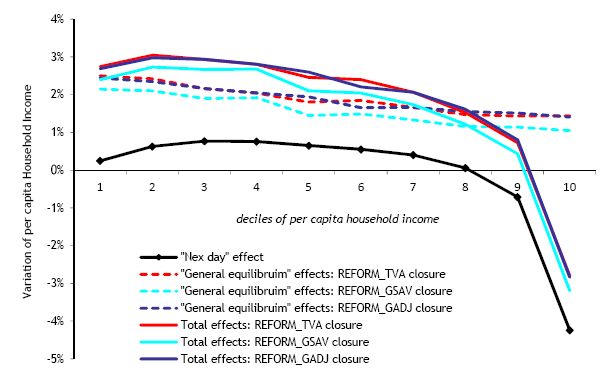

After-tax per capita household income by decile and type of microsimulation. Full reform (variation w.r.t base).
7. Concluding remarks
First, it is important to remark that we find significant general equilibrium effects from the full implementation of the 2007 tax reform. Taken together, they tend to reinforce the progressive nature of the “next day” effects of implementing its main policy, i.e. the introduction of a direct personal income tax with higher progressive marginal rates to replace the previous wage and pension tax. Although this is an expected result, it reinforces the importance of evaluating these types of macro reforms using methodologies that account for potential reallocation of resources due to changes in prices of goods and factors due to the policy.
Second, the main results relating to the effects of the full implementation of the reforms on aggregate economic activity, employment, poverty and inequality are robust to the alternative assumptions about government closure, although there are clear differences regarding the absorption structure and public-private shares of investment, in addition to possible dynamic effects that are not captured in this analysis. The results are robust to variations in key parameters.
An important result is that the full reform increases GDP and employment, even though it actually increases the tax burden. In other words, when government revenues increase due to the tax reform (and allow an increase in either government provision of public services or government savings), the reform also results in employment and wage growth and reduced unemployment, generating positive general equilibrium effects on average household income and poverty. This obviously does not mean that the government’s use of additional revenue is irrelevant. The simulations that alter either government consumption or savings accounts tend to crowd out private consumption or savings, with probable future negative effects on private capital accumulation. When the government budget is held fixed and additional reductions of the VAT rate are allowed, the reform generates the most positive effects in relation to economic activity, poverty and inequality.
This result is linked to the fact that the reform generally reduces or eliminates taxes on some goods and factors and harmonizes tax rates across categories for others. This is done through the elimination of the intermediate consumption tax and the health tax, and reductions in the VAT and ECSS, with any revenue losses being compensated for by an increase in direct taxation. Reduction, elimination or harmonization of these taxes tends to reduce price distortions of goods and factors. In a context of perfect factor mobility across economic activities, this leads to a better reallocation of resources, stimulating an expansion of economic activity.
Although direct taxation on household income could also be distortionary because of the efficiency loss associated with substitution between labor and leisure, the simulated models suggest that the proposed shift towards direct taxation in Uruguay is desirable from an efficiency perspective. Despite an elastic labor supply in the model, the final simulated changes in participation rates were insignificant and robust to sensitivity analysis. However, progressive marginal tax rates on household income could also have negative impacts on private savings, with negative implications for dynamic capital accumulation. In the long run, non-linear marginal rates on income may also induce negative effects on human capital accumulation by lowering the wage premium for the more educated. These aspects are not considered, and they would require further analysis using a dynamic framework.
We also find that the general equilibrium effects of the full reform include an increase in aggregate disposable household income, which compensates for the reduction obtained by the application of the personal income tax ignoring other components of the reform and economic agents’ responses to the reform. The magnitude of the general equilibrium effects on poverty indicators is significantly greater than the “next day” effects. The 1-point reduction of the Gini inequality coefficient is entirely due to the progressive nature of the personal income tax: households in the richest decile are the clear “losers” from the reform. However, the general equilibrium effects of the full reform do not play a significant role in this regard.
Finally, the results also indicate that VAT rates could be lowered further to make the reform budget neutral. When the full reform is compensated by changes in VAT rates, the VAT rates could be lowered by an additional percentage point, to 21% for the basic rate and 9% for the minimum rate. As budget-neutrality with additional reductions in the VAT rate generates the larger positive effects on aggregate economic activity, poverty and inequality, this suggests that further reductions in VAT rates are desirable both with respect to efficiency and equity.
Footnotes
1.
The BPC is a unit of account that is adjusted according to average wage growth. The nominal value of the BPC was 1636 Uruguayan pesos (approx. 74 dollars) in January 2007.
2.
A detailed description of all the equations is available from the authors upon request.
3.
Results are available from the authors.
4.
Also note that the CGE model does not endogenize this aspect of the labor market.
5.
This result is highly dependent on the assumption of perfect competition. For the case of Uruguay, a small open economy, this assumption is reasonable for the tradable sectors (especially manufacturing and primary activities). However, imperfect competition would probably be a more realistic assumption for some non-tradable sectors. In these cases, the reduction in VAT rates could be entirely (or mostly) captured by firms and thus not lead to efficiency gains.
6.
Results are available from the authors.
References
-
1
‘Taxation Reforms: A CGE-Microsimulation Analysis for Pakistan’. MPIA Working Paper 2010-12‘Taxation Reforms: A CGE-Microsimulation Analysis for Pakistan’. MPIA Working Paper 2010-12.
-
2
‘The impact of the Indonesian income tax reform: A CGE analysis’Economic Modelling 31:492–501.
-
3
‘Wage inequality and the distribution of education: a study of the evolution of regional differences in Metropolitan Brazil’Journal of Development Economics 36:117–143.
-
4
‘The design of tax structure: direct versus indirect taxation’Journal of Public Economics 6:55–75.
-
5
‘Impacto distributivo de la reforma impositiva’Draft prepared for Poverty and Social Impact Analysis (PSIA).
-
6
Modelling labor markets in CGE models. Endogenous labor supply, unions and efficiency wagesMontreal, PEP – CIRPEE – Université Laval.
- 7
- 8
- 9
-
10
‘MIDD: the microeconomics of income distribution dynamics. A comparative analysis of selected developing countries’Paper presented at the 2001 Latin American Meeting of the Econometric Society.
-
11
‘Fast development with stable income distribution: Taiwan, 1979-1994’Review of Income and Wealth 43:139–164.
-
12
An estimation of wage curve for UruguayMimeo: Departamento de Economía de la Facultad de Ciencias Sociales.
-
13
The Impact of Namibia’s Income Tax Reform: A CGE Analysis. AGRODEP Working Paper 0020Washington, DC: International Food Policy Research Institute.
-
14
‘Linking CGE and microsimulation models: a comparison of different approaches’International Journal of Microsimulation 3:72–91.
-
15
‘Endogenous labor supply with several occupational categories in a bi-regional CGE Model’Regional Studies, Taylor and Francis Journals 44:1401–1414.
-
16
‘The Case for a Progressive Tax: From Basic Research to Policy Recommendations’Journal of Economic Perspectives 25:165–90.
- 17
-
18
‘Sistemas tributarios alternativos y su impacto en la distribución del ingreso y en la oferta laboral. Una aproximación comportamental para el caso uruguayo’Revista Quantum, VI, 1.
-
19
Armington Elasticities: Estimates for Uruguayan Manufacturing SectorsDepartamento de Economía, Universidad de la República Serie Documentos de Trabajo.
-
20
Liberalization, inequality and poverty. Latin America and the Caribbean during the ninetiesLiberalization, inequality and poverty. Latin America and the Caribbean during the nineties, ed., UNDP.
-
21
‘An analysis of South Afica’s value added tax’. World Bank Policy Research Working Paper 3671‘An analysis of South Afica’s value added tax’. World Bank Policy Research Working Paper 3671, August.
-
22
Distribución del ingreso y crecimiento: La expansión del mercado interno vía la redistribución de los ingresos: un ejercicio de simulación para la economía uruguaya’, Trabajo de investigación monográfico para la obtención del título de Licenciado en EconomíaMontevideo: UdelaR.
-
23
The Uruguayan tax structure and its incidence on income distributionMontevideo: Fundación de Cultura Universitaria.
-
24
Políticas públicas para el desarrollo humano. ¿Cómo lograr los Objetivos de desarrollo del Milenio en América Latina y el Caribe?‘Uruguay’, et al, Políticas públicas para el desarrollo humano. ¿Cómo lograr los Objetivos de desarrollo del Milenio en América Latina y el Caribe?, Santiago, PNUD y Uqbar editores.
-
25
¿Quién se beneficia del libre comercio? Promoción de exportaciones y pobreza en América Latina y el Caribe en los 90‘Uruguay: export growth, poverty and income distribution’, et al, ¿Quién se beneficia del libre comercio? Promoción de exportaciones y pobreza en América Latina y el Caribe en los 90, New York, UNDP.
-
26
Microcomputers in Policy Research‘A standard computable general equilibrium (CGE) model in GAMS’, Microcomputers in Policy Research, 5, Washington, DC, IFPRI.
-
27
The tax system and income distribution in Uruguay. Monographic Research. Facultad de Ciencias Económicas y Administración- Universidad de la República, MontevideoThe tax system and income distribution in Uruguay. Monographic Research. Facultad de Ciencias Económicas y Administración- Universidad de la República, Montevideo.
-
28
Crisis and Income Distribution, A Micro-Macro Model for IndonesiaCrisis and Income Distribution, A Micro-Macro Model for Indonesia, The World Bank (mimeo).
-
29
‘Direct or indirect tax instruments for redistribution: short-run versus long-run’Journal of Public Economics 88:503–518.
-
30
‘A general equilibrium calculation of the effects of differential taxation of income from capital in the U.S.’Journal of Public Economics1 (3–4) pp. 281–321.
-
31
‘General equilibrium with taxes: A computational procedure and an existence proof’The Review of Economic Studies pp. 475–489.
-
32
‘Applied general-equilibrium models of taxation and international trade: an introduction and survey’Journal of Economic Literature pp. 1007–1051.
-
33
The effects of increasing openness and integration to the Mercosur on the Uruguayan labor market: a CGE modelling analysis. MPIA Working Paper 2006-06Canada: Laval University.
- 34
Article and author information
Author details
Acknowledgements
This work was carried out with financial and scientific support from the Partnership for Economic Policy (PEP), with funding from the Department for International Development (DFID) of the United Kingdom (or UK Aid), and the Government of Canada through the International Development Research Center (IDRC). Mery Ferrando provided very helpful assistance. We are very grateful to Bernard Decaluwé, Ismael Fofana, Veronique Robichaud, Martin Cicowiez and John Cockburn for their useful comments and suggestions. All remaining errors are ours.
Publication history
- Version of Record published: April 30, 2016 (version 1)
Copyright
© 2016, Llambi et al.
This article is distributed under the terms of the Creative Commons Attribution License, which permits unrestricted use and redistribution provided that the original author and source are credited.