Estimating and simulating with a random utility random opportunity model of job choice. Presentation and application to Belgium
- Department of Economics, KU Leuven, Belgium
- Federal Planning Bureau, Belgium
- Article
- Figures and data
-
Jump to
- Abstract
- 1. Introduction
- 2. The RURO model
- 3. Likelihood function, functional form, and estimation
- 4. Data
- 5. Estimation results
- 6. Fit and behavioural response
- 7. Education and labour market participation
- 8. Conclusion
- Footnotes
- A1. Poisson processes
- A2. Likelihood: the case of couples
- A3. Coefficient estimates
- References
- Article and author information
Abstract
We present the Random Utility Random Opportunity (ruro) model of job choice (Aaberge, Dagsvik & Strøm, 1995, and Aaberge, Colombino & Strøm, 1999) and report estimation results from an application of a version of that model on Belgian data (eu–silc 2007). We discuss the effect of education level on the intensity of preference for leisure relative to consumption, on the intensity of job offers, and on the wage offer distribution. Finally, we report simulation results with respect to the impact on labour market participation by letting the male catch up the arrears in educational attainment they currently have with respect to females.
1. Introduction
The purpose of the present paper is to explain and illustrate how to estimate and simulate with a Random Utility Random Opportunity (henceforth ruro) model of job choice (see amongst others Dagsvik & Strøm, 1992, 2003, and 2006, Aaberge, Dagsvik & Strøm, 1995, Aaberge, Colombino & Strøm, 1999, and Dagsvik, Locatelli & Strøm, 2006 and 2007).1 These type of models, first developed in an abstract setting by Dagsvik (1994), try to understand individual heterogeneity in choice behaviour as a combined effect of differences in preferences and opportunities. Contrary to the classical discrete choice models of labour supply (Van Soest, 1995), this approach provides a structural framework for assessing the impact of both, labour supply and labour demand side effects, on labour market participation.
Traditionally, preferences in labour supply models capture the extent to which an individual is willing to trade-off leisure for consumption. It may however deserve recommendation to take into account also other aspects influencing the choice between alternative leisure activities and available jobs, such as social relations involved, challenge of the tasks, security and health, recognition, and societal relevance. But these factors are not easily observable by the analyst. It was one of the contributions of the development of probabilistic choice and random utility models, as developed by respectively Luce (1959) and McFadden (1973), to integrate these additional determinants of preferences as a non-systematic element, affecting the utility obtained from different available alternatives. By non-systematic it is meant that such factors are uncorrelated with, and therefore cannot be explained by observable characteristics. Random utility models have been applied to labour supply behaviour since (Van Soest, 1995). They replaced the traditional continuous choice approach to labour supply behaviour (see Hausman, 1985, for a review of this traditional approach), which faced difficulties in deriving tractable closed form solutions of labour supply functions, in the presence of non-linear budget sets. Indeed, many personal income tax systems, such as e.g. a minimum income guarantee associated with a linear earned income tax, create non-convexities in the budget set (the available bundles of consumption and labour time a person can chose from), leading to discontinuities and non-uniqueness of the optimal choice in function of wage variations. These phenomena are more easily treated in a discrete choice set-up, which is the approach taken by both, probabilistic choice and random utility models.
The random utility model is however still limited in scope. Interindividual differences in the availability of alternatives from which a person can choose, are exogenous to the model. Applied to job choice, differences in individual budget sets stem exclusively from wage differences and differences in unearned income. In a static model, it is indeed reasonable to assume that unearned income differences are exogenous, and do not depend on individual choices. But in standard random utility models also wages are exogenously fixed individual characteristics, reflecting a person’s productive capacities.2 This is unattractive. Productive capacities can in many cases not be determined appropriately, when considered separately from the specific job in which these capacities are exhibited. Moreover, it is quite unnatural that all available job offers, even when perfectly suited to a person’s capacities and skills, would pay the same wage. Besides the question of the meaning and determination of the wage, it is also highly unlikely that persons can completely freely fix the number of hours they will work, due to organisational limitations of the production process and social life.
It is exactly these type of frictions in the choice process which are taken into consideration by ruro models, as an additional factor, next to preferences, to understand choice behaviour. Job offers are considered as packages of wages, labour time regimes, and a number of other attributes (Dagsvik & Strøm, 1992, 2003, and 2006, Aaberge, Dagsvik & Strøm, 1995, and Aaberge, Colombino & Strøm, 1999). These other attributes (challenge, safety and security, esteem and recognition, appreciation of colleagues, responsibility...) are however difficult to observe, especially as far as it concerns the degree of job satisfaction they can provide to a person. Therefore, the individual specific availability of suitable jobs is thought of as the result of a stochastic process of job offers. The impact of explanatory variables on the intensity with which job offers arrive to a person according to that process, is estimated jointly with individual’s preference characteristics. Not only the intensity with which job offers arrive, but also the availability of, according to a person’s own judgement, attractive nonmarket alternatives to spend time, is individually specific. Limited physical abilities might impede someone who likes to walk outside, to do so. Choosing under such circumstances between sitting in front of a liquid crystal screen, reading books, or accepting a job, that person might opt for the latter, while the reverse might happen for someone with similar preferences, but in good physical shape. The RURO model also allows for individual heterogeneity in restrictions on available labour time regimes, even though the effect of these type of restrictions are difficult to identify from the contribution of preferences.
The ruro model is not the only one that embodies restrictions on the choice set into a labour supply model (see, amongst others, Altonji and Paxson, 1982 and 1992, Van Soest, Woittiez and Kapteyn, 1990, Tummers and Woittiez, 1991, Dickens and Lundberg, 1993, Bloemen, 2000 and 2008, Ham and Reilly, 2002, and Beffy et al., 2016). It must be added that the inclusion of dummies for part time and full time work in the discrete choice model of Van Soest (1995), to improve the fit, is in fact a simplified reduced form approach of earlier work with Woittiez and Kapteyn (Van Soest, Woittiez & Kapteyn, 1990) which models hours restrictions more explicitly. But the RURO model is the first one that derives these restrictions from an explicit model of a job arrival process, and stresses the individual heterogeneity, both observed and unobserved, of the availability of job offers suitable to the capacities of individual agents.
In the present paper we present estimation results of a version of the RURO model of job choice on Belgian data (eu-silc 2007).3 In our data the unemployment rate of lowly educated males is more than 20%, as compared to somewhat more than 4% among highly educated males, and a general unemployment rate of 10%. For females these figures are almost 50% for the lowly educated, 8.5% among highly educated, and almost 24% in general. We illustrate the potential contribution of the different components of the model to explain these figures: the relative intensity of preference for leisure, the intensity of suitable job offers, and the wage offer distribution. Next, we report simulation results assessing the impact on labour market participation of a scenario in which males’ education level largely catches up that of females.4
In Section 2 we give a self–contained exposition of the ruro model. Section 3 discusses the resulting likelihood function and explains the estimation method. We also devote some time to explain how the estimated model can be used for simulation purposes, both to assess the fit, or to predict the effects of counterfactuals such as tax reforms. Technical issues are relegated to the Appendix. The data are presented in Section 4. Section 5 contains the estimation results. We give graphical representations of the estimated preferences and opportunities side of the estimated model. In Section 6 we investigate the fit of the estimated model, and its behavioural implications. Finally, Section 7 presents the results of the simulation exercise with respect to the effects of a counterfactual educational attainment level. Section 8 concludes.
2. The RURO model
In the present section, we present a version of the general ruro model applied to job choice as developed by Dagsvik and Strøm (1992, 2003, and 2006), Aaberge, Dagsvik and Strøm (1995), and Aaberge, Colombino and Strøm (1999). We first illustrate how the ruro model extends the choice problem of traditional labour supply models from a question of trading off leisure against consumption towards a model of job choice against other non–market alternatives of time use (Subsection 2.1). Then, we discuss the preference part of the model (Subsection 2.2). Finally, we expose the modelling of opportunities (Subsection 2.3).
2.1 Opportunities and jobs
In general, the ruro model is an economic model of human choice behaviour. Human decision makers are assumed to choose the best element from a set of choice possibilities or opportunities, where ‘best’ is defined in terms of preferences (or, vice versa, preferences are derived from observed choice behaviour as that objective which would be maximised given those choices). Applied to job choice, the set of opportunities is to be thought of as a set of possible activities a particular individual might choose to execute. Some of these activities are rendered available through job offers. These job offers will be indexed by j, where the variable j belongs to an index set, say J. A job offer stipulates an amount of labour time to be supplied when accepting the offer, say h, and pays a wage, w. It is assumed that this wage can be expressed in units of time effectively spent on the job, so that (gross) revenues earned by the job equal the amount of time spent on the job times the wage.
Gross earned labour income is then equal to wh. Gross earned labour income together with some other characteristics, say xf, among which non-earned gross income (exclusive of transfers), determine the outcome of the gross to net (disposable) income function c = f (w, h;xf), where c stands for consumption, which in a static model as the present one coincides with disposable income.5 That is, saving is considered as part of consumption. The function f converts gross income components into net disposable income, by subtracting taxes to be paid and adding transfers and subsidies. Usually, the generation of disposable income is constructed from raw data on gross income, labour time and other characteristics, by means of a microsimulation model.
Besides time spent on the job and the remuneration, jobs exhibit a number of other characteristics such as degree of responsibility, variation and challenge of the tasks, safety, healthiness, physical effort, stress, relation with colleagues and superiors. Preferences over these non–pecuniary attributes affect job choice.
One might also decline all job offers. Evidently, not executing a formal job does not require any time to be spent on the formal labour market (h = 0), and is assumed not to pay a wage (w = 0). A person who does not work, receives a net transfer (that is after deducting income taxes to be paid from her replacement income) equal to f (0, 0;xf). In that case, time is spent on executing some of the available non–market opportunities. However, the set of activities6 one has alternatively available is not the same for all individuals, neither is the extent to which a particular alternative is available. When living in a small town, attending concerts, theatre or visiting museums is certainly not as easy as for big city dwellers. If you are in a wheel chair, hiking is not an option. Which of the available non–market activities will be chosen, in case no job offer is accepted, again depends on preferences (or, vice versa, what one chooses to do allows to derive something on the shape of preferences that person supposedly has). Non–market alternatives will be indexed by i, belonging to the index set I. The index sets for jobs and non–market alternatives respectively, are disjointI ∩ J = Ø. We will also use the index variable z to indicate an alternative in general, that is either a job or a non–market alternative. So, z ∊ Z := I ∪ J. To be really precise, an index z refers to a set of activities. If this set involves one or more jobs, the index z will belong to J, while it belongs to I otherwise. An alternative including several part time jobs is described by the total number of hours these jobs involve and the hourly wage these pay together (calculated as earnings divided by total hours).
2.2 Random utility
In the model, preferences are defined over the number of hours h spent on jobs (which is zero if one chooses not to accept any job offer), consumption, c, and a set of other attributes that a job or certain non–market activities possess, and that a person might care for. These other attributes are not observed by the researcher.
The observable bundle of characteristics an alternative z ∊ Z exhibits, is denoted by (C(z), H(z)), where C(z) refers to the individually specific net disposable income resulting from executing activities indicated by z, and H(z) to the labour time involved by the set of activities indicated by z. The utility derived from these observable characteristics is denoted by V (C(z), T − H(z); xV), where xV are the specific values of a set of preference shifters for the individual under consideration, and T denotes the number of time units available in the period over which labour time h is registered (e.g. 168 hours a week, if labour time is expressed in hours worked per week). It is assumed that the econometrician can derive some evidence on the shape of the function V on the basis of observations on (C(z), T − H(z)) and xV. So, no individual preference differences apart from those explained by observable characteristics xV, are allowed for in this part of the utility function, and V is therefore called the systematic part of the utility function, and, hence, of preferences.
Since the other attributes besides disposable income and labour time are not observable, their contribution to utility will be specified as a random term. Thus, the utility generated by these attributes of set of activities z, is denoted by the random variable ε (z). It is assumed that this utility from non–pecuniary attributes, ε (z), enters overall utility of an alternative z in a multiplicatively separable way from the systematic part of the utility function. In order to make sense, this requires both, the systematic part of the utility, and the random term, to be non–negatively valued functions.
In summary, the total utility derived from picking an alternative z ∊ Z, say U (C(z), H(z), z;xV), equals:
As c = f (w, h;xf), the systematic part of the utility function, V (c, T – h;xV), induces a utility function, say Ψ, defined over hours worked on the formal labour market, h, and wage, w:
Consequently,
where W (z) is the wage paid by activity z. More in particular, for someone not accepting any job offer, and choosing an alternative i ∊ I, utility equals:
The domain of the systematic part of the utility function in the wage-hours space, Ψ(·; xV, xf), is [0, ∞) × [0, T).
From now on we will drop the conditioning variables xV and xf in the systematic part of the utility functions.
2.3 Random opportunities
Both, jobs and non–market activities, are not equally available to all individuals. This is captured by the notion of intensity with which alternatives are rendered available to a specific individual. The probability to receive a job offer as a civil engineer, for someone who has only completed secondary school, is e.g. zero. Something similar holds for non–market activities: they are not all equally available to all agents. Someone having lost her legs will not be able to run (or not in the same fashion as before), though she might continue to be fond of it.7
The intensity with which a job is offered to an individual depends on a number of personal characteristics, such as skills, education, experience, and on the characteristics of the job itself, more specifically, the wage, the labour time regime of the job, and its other attributes. For the sake of simplifying notation we will drop the individual conditioning variables.
In Equation (2), preferences were defined over the continuous set of all possible amounts of time spent on the jobs. In the real world, however, jobs requiring a non–rational number of hours a week, are not available. Be it alone to organise the production process, it might sometimes be required to have a number of people working together during a fixed number of hours. So, in practice, full-time, three-quarter time, half time, one-quarter, or 20% jobs are more densely offered than other labour time regimes. Let g2(h) be the density with which jobs requiring h hours of labour supply, are rendered available to a specific individual. Similarly, jobs pay different wages. By g1 (w|h) we denote the density of jobs paying a wage w, within the class of job offers available to a specific individual, that require h hours of work.
Persons do not only care for the wage a job pays, and the number of hours to be worked, but also for other job attributes. From a behavioural theoretic point of view (see Equation 1), these are only important in as far as they yield a specific value for the multiplication factor in the utility function for those alternatives. Two jobs, j1 and j2 say, paying the same wage and requiring the same amount of hours, with attributes yielding the same value of the multiplication factor in the utility function for those alternatives, that is ε(j1) = ε(j2), are thus, according to the behavioural model of Equation (1), equivalent to each other in the present model, and therefore will be considered as the same opportunity. The variable indicating the value of this multiplication factor is denoted by ν.
The intensity with which job offers yielding a value ν, are arriving to a specific individual is denoted by λ1 (ν).8 We assume the following functional form for λ1:
where q is a measure for the demand by the market for capacities and characteristics an individual possesses, relative to those capacities which are currently unsolicited by jobs, and which are therefore called non–market opportunities.
The functional form of λ1 implies that attributes which are particularly disliked (yield a very small value for ν) are excessively abundant, while those that are particularly liked (yielding a very high value of ν), are extremely scarce. This functional form guarantees independence of irrelevant alternatives in the probability of choosing jobs (Dagsvik, 1994).
Now, let ℋ be the set of all possible labour time regimes of jobs offered in the market, and W the set of possible wage offers. Wages can obtain any positive value. Let ℬ := ℬh × ℬw be the Cartesian product of a measurable subset of labour time regimes ℬh ⊆ ℋ, and wage offers ℬw = (0, w), for some positive w. The arrival of job offers9 to an individual, is modelled by an inhomogeneous spatial Poisson process. Events are job offers that are characterised by a labour time regime h, a wage offer w, and the utility that can be derived from other attributes ν. The intensity parameter of this Poisson process is equal to g2 (h)g1 (w|h)λ1 (ν). Define next the set of job offers specifying a labour time regime t £ ℬh, paying a wage r lower than w (that is r £ ℬw), and which will yield a utility level at least equal to u, as Uh,w,u := { (t, r, ν) £ ℬh × ℬw × ℝ+|Ψ(r, t) ν ≥ u}, and define:
Let N(ℬ, u) be the number of job offers with a wage r belonging to ℬw, the number of hours to be worked in ℬh, and yielding a utility level larger than or equal to u. The probability for an individual to be offered n such jobs is under the present assumptions governed by a Poisson distribution, and is thus equal to:
Thus, Λ1 (Uh,w,u) can be interpreted as the expected number of job offers with labour time regime, wage, and utility level in Uh,w,u.
As the arrival of job offers is modelled as a stochastic process, the utility level obtained from jobs with a wage in ℬw, number of hours to be worked in ℬh, and other attributes yielding a value for the multiplicative factor equal to ν, is a random variable too, denoted by Uℬ. The probability that Uℬ is less than u, denoted by P (Uℬ < u), equals the probability that the number of available alternatives with utility larger than or equal to u, is zero. From Equation (7) with n = 0, it thus follows that:
Hence, Uℬ turns out to be Fréchet distributed with location parameter μ = 0, scale parameter
and shape parameter α = 1.10
The derivation of this distribution is equally valid for any (measurable) subset ℬ of the space of possible working times and wage combinations, job offers might exhibit. More in particular, it holds for the complement of ℬ in the set of all possible working time wage combinations, defined as . It follows that the random variable Uℬc, denoting the utility level derivable from possible job offers with working time wage combinations in ℬc, is Fréchet distributed with location parameter μ = 0, scale parameter
and shape parameter α = 1.
The distinguishing value of different potential non–market activities, is completely absorbed by the different values of the multiplication factor in the utility function they generate. Indeed, the systematic part of the utility function is for all non–market alternatives equal to Ψ(0, 0). As for jobs with the same wage and required labour input, two non–market activities, i1 and i2 say, with attributes yielding the same value of the multiplication factor in the utility function for those alternatives, that is ε(i1) = ε (i2), are from a behavioural theoretic point of view equivalent to each other, and will therefore be considered as one and the same opportunity. For the same reason as in the case of job offers, it will be assumed that leisure activities which are particularly disliked, are abundantly available, while those that are intensely desired, are rather difficult to obtain. The intensity with which nonmarket activities yielding a multiplication factor equal to ν, denoted by λ0 (ν), are accessible to an individual, is thus assumed to be equal to:
Let ℰu be the set of values for ν such that non–market activities yield at least a utility level larger than or equal to u: ℰu = {ν ∊ ℝ+|Ψ(0,0)ν≥ u}. Define Λ0(ℰU), as:
If one assumes that λ0 is the intensity measure of an inhomogeneous spatial Poisson process, then the number of non–market alternatives that yield a utility level of at least u, available to a person, is Poisson distributed (see Appendix A1). Let the number of available non–market activities yielding a utility level of at least u, be denoted by N(Ψ(0,0) ν ≥ u). The probability that N(Ψ(0,0)ν ≥ u) = n, is, according to the Poisson distribution, equal to:
The value of Λ0 (ℰu) equals the expected number of non–market opportunities available to an individual, yielding a utility level at least equal to u. The higher the value of Λ0 (ℰu), the more skewed to the right this distribution becomes, that is, the higher the probability that the number of available non–market alternatives yield a utility level of at least u is relatively big.
The probability that all available non–market alternatives to an individual, yield a utility level lower than u, equals the probability that the number of available alternatives with utility larger than or equal to u, is zero:
From the last equation, it can be concluded that the utility that can be derived from the available non–market alternatives, which is a stochastic variable denoted by U0 = Ψ (0,0) ν, is Fréchet distributed with location parameter μ = 0, scale parameter σ0 = Ψ(0,0), and shape parameter α = 1. This will prove useful when formulating the likelihood function in the next section (Section 3.1).
3. Likelihood function, functional form, and estimation
3.1 Likelihood function
Now we turn to the behavioural implications of the model explained in Section 2. From the available job offers and non–market opportunities, a person will choose that alternative she likes most. The probability that this will be an alternative including a job offer with a working time wage combination in the set ℬ, is equal to the probability that Uℬ > max {U0, Uℬc}.
As the processes governing the arrival of job offers and non–market opportunities are assumed to be independent, the probability that Uℬ (the utility from a job offer with a labour time and wage combination in ℬ) is equal to or greater than max {U0, Uℬc} is equal to the product of the probability that Uℬ is greater than or equal to U0 and the probability that Uℬ is greater than or equal to Uℬc. That amounts to:
In a similar fashion it can be derived that the probability to choose a non–market alternative, is equal to the probability that U0 is equal to or greater than Uℬ∪ℬc, which is equal to:
An additional assumption for identification is the independence of the wage offer distribution from the hours specified by the job offers. That is g1 (w|h) = g1 (w), ∀h ∊ ℋ.
The likelihood that an individual will choose one particular job offer requiring labour time h, and paying a wage w, can thus be obtained from Equation (15):
Similarly, the likelihood an individual’s most preferred non–market alternative is preferred to any of the job offers, equals:
We exclusively concentrated on individual decision makers. The model can be extended to the case of households consisting of couples (with or without children), if one is willing to assume a unitary decision making model. We provide this extension in Appendix A2.
It is worthwhile to compare the likelihood function (15)–(15’) with what is obtained in a random utility function based upon discrete choice of labour time regimes (such as in Van Soest, 1995). In this approach, the wage a person obtains, is, apart from measurement problems (see note 2), a fixed individual characteristic reflecting that person’s productivity. Choice of labour time is free but limited to a discrete set {hi;k = 1,2,..., K}. Under the assumption that the stochastic parts of the utility functions are Fréchet distributed, the likelihood (probability) to observe an individual choosing a labour time regime hi equals:
The difference with (15)–(15’) is twofold. In the ruro model utilities are weighted with the intensity with which alternatives are rendered available to an individual. Next, the wage is part of the job offer. Consequently the denominator sums over all possible pairs of wages and labour time regimes (w, h), job offers contain, and not only over possible labour time regimes for a given wage.
3.2 Identification
Some parts of the model are non–parametrically identified. A fuller treatment of this issue is provided in Aaberge, Columbino and Strøm (1999), the working paper version of Dagsvik and Strøm (2006) (See Dagsvik & Strøm, 2004), and Dagsvik and Jia (2016). The main line of argument for identifying the wage offer distribution from preferences runs as follows. Isolate two observationally equivalent groups of individuals in the population, supplying different number of hours, say h1 and h2, for the same wage w. The relative proportion of these groups in the population is φ (w, h1) / φ (w, h2), which according to the model in Equation (17) reduces to:
Doing this for different levels of wages, allows to identify the function Ψ (w, h) g2 (h). Looking then at persons performing the same number of hours, but accepting different wages, w1 and w2 say, gives:
As Ψ (w, h) g2 (h) was already identified in the previous step, it is now possible to identify g1 (w), using the fact that it is a density, and thus that ∫w∈W g1 (w) d w = 1.
Then, consider an observationally equivalent group of persons in the population. Some of them will be engaged in a formal job, and some of them not. The relative proportion of those groups in the population are:
As Ψ is a utility function, we can normalize the value of Ψ (0,0), which allows to identify q from this equation. In our empirical application, we tried to improve upon the non–parametric identification of q by introducing an exclusion restriction. More specifically, a group specific unemployment rate11 is added as an explanatory variable for q. We assume that this variable does not affect individual preferences, but, obviously, it has some relation with labour demand.
The utility function Ψ (w, h) and the distribution of offered labour time regimes g2 (h) are however not separately non–parametrically identified. One way out is to give a more fundamental justification of the functional form used for preferences. For example, Dagsvik and Røine Hoff (2011) and Dagsvik (2013) give a non–parametric justification of the preferences embodied by the Box-Cox type of utility functions that we will use (see the next section).
Moreover, it can be argued that the occurrence of peaks in the distribution of the number of hours worked, as observed in many datasets, around half time, three quarter time and full time work, are not easily explained by the traditional way preferences are shaped in economics, neither by the kinks in the shape of the budget set caused by different tax structures.
3.3 Functional forms
In the present section we present the functional forms of the different components of the model that will be used in the empirical application in Section 5.
At the preference side,
the systematic part of the log utility function for singles is of the Box-Cox type: ln , with αc, αh < 1. Intensity of preferences for leisure is increasing (decreasing) in an element of xV, if the associated parameter of βh is positive (negative).12 The exponents, ac and ah, determine the curvature of the indifference curves in terms of labour time and consumption (that is, while keeping other attributes affecting preferences fixed). The lower these are, the less substitutable leisure and consumption are;
for couples, a unitary decision model is assumed, but spouses’ leisure time is considered to be an assignable good. So, the systematic part of preferences is defined over consumption and each spouse’s leisure time. Partner’s time endowments are equal. An interaction term capturing potential complementarities between partners’ leisure time, is added to the utility function:
(23)with αc,g, αhi < 1 (i = 1,2). The interpretation of the exponents and the (i = 1,2) remains the same as for singles; in addition, βh1,h2 > (<)0 means that partners’ leisure are complements (substitutes).
At the opportunity side,
the log of the intensity of job offers relative to the availability of non–market alternatives is linear in the covariates: ln . The vector xopp resumes covariates that might affect the job offer intensity, and should contain a constant term. The coefficient associated to this constant term is denoted by ηq,0;
the wage density g1 (w; xw) is assumed to be lognormal:
. It is dependent on covariates xw that might affect the wage offer distribution;
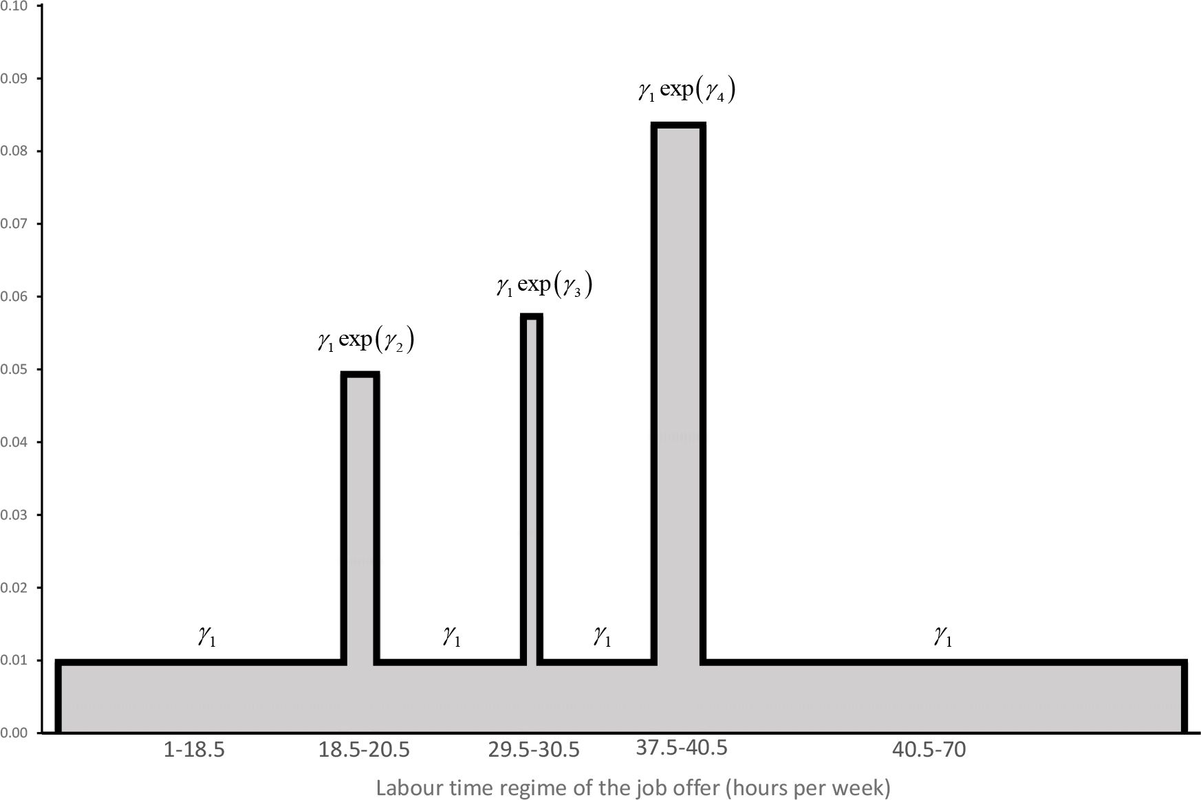
the distribution of the labour time regimes offered, is piecemeal uniform. There are a number of, say K, peaks, indexed by k = 1,2,..., K, around which the bulk of the job offers’ labour time regimes are concentrated (typically around half time, that is 18.5 to 20.5 hour a week in our application, three quarter time, or 29.5 to 30.5 hours a week, and full time, or 37.5 to 40.5 hours). The lower and upper bound of peak k (k = 1, 2,..., K) are denoted by respectively and . There is a lower limit, Hmjn, below which job offers are not considered to belong to the formal labour market (fixed at one hour a week in the application below); and an upper limit of labour time spent on formal jobs, denoted by Hmax, and fixed at 70 hours per week in our application. This results in the following density function:
(24)An example of such a distribution function is given in Figure 1. In our application, the only covariate in xh allowed to affect this function is the sex of the person .
3.4 Estimation
To estimate the parameters governing preferences, the relative intensity of market over non–market alternatives, and the distribution of wage offers and labour time regimes, a likelihood function, say ℒ, is constructed on the basis of Equations (17) and (18’) (for the case of the couples, see Equation (18”) of Appendix A2). The individual contributions of a single to that likelihood function are composed of the likelihood that the observed choice is the most preferred one, reflected in Equations (17), or (18’), depending on whether the observed choice involves participation on the formal labour market executing a job (or set of jobs) requiring h hours of work, and paying a wage w, or whether it is the non–market alternative. In these expressions, the numerator is thus evaluated at the actually observed choice, when constructing the likelihood function. Similarly for couples, the first, second, third, or fourth equation in (15”) (in Appendix A2) applies, dependent on whether both partners, only partner j (j = 1, 2), or none of both actually are engaged in formal jobs.

Peak distribution for labour time regimes.
In practice, we do not observe the set of wage offers, W, nor the offered labour time regimes, ℋ. Therefore, a set of alternatives in the space of wages and labour time regimes is sampled from a prior density function, say ℙ (w, h). Denote the set of sampled combinations of wage offers and labour time regimes, possibly including the non–market alternative, by D. The observed choice (wobs, hobs) is to be always included in the sampled choice set. From the sampling densities ℙ (w, h), the likelihood to sample a set D given that the observed choice equals (wobs, hobs), can be constructed.13 It is denoted by P (D | (wobs, hobs)), and it equals:
Recall that the probability (density) that a job paying a wage w, and requiring a number of h hours to be worked, would be optimal given a choice set C := {0,0} ∪ W } ℋ, was derived in Equations (17), and (18’) if the non–market alternative would be the most preferred option. The unconditional probability to sample a choice set D, denoted by Π (D), can thus be written as:
Using Bayes’ law, the probability (density) to observe an agent choosing a job offer that pays a wage wi, and requires hi, hours of labour time from the sampled set D, thus equals:
Using Equations (25) and (26), we can thus reformulate the simulated likelihood to observe someone choosing an alternative (w, h) from a choice set D sampled according to the prior ℙ (w, h), as:
The corresponding expression for choosing the non–market alternative equals:
One further normalisation issue is in order. Note that the constant term of the q (xopp)–function, exp(ηq,0), occurs in any term of the likelihood where γ1 appears (that is, in those terms of the sum pertaining to a job offer on the formal labour market, (w, h) : w, h > 0), and each time these terms appear as a product. Therefore both, ηq,0 and γ1, cannot be estimated separately. But γ1 is still identified by the identity:
This means in practice that one does not estimate all the parameters in the likelihood (23) (respectively 23’), but rather reduces these equations to:
where:
For the likelihood to choose a non–market alternative, this becomes:
One is able to back out an estimate of ηq0 by using Equation (30). Indeed, subtracting ln (with , the estimated value of γ1 from applying Equation (30) using the estimates for 7k+1, for k = 1,2,..., K) from the estimated constant of ln .
We used the following specification of ℙ (w, h) for constructing a choice set D: wages are sampled from a lognormal distribution with parameters m and ς, labour time is sampled from the uniform distribution on the [Hmin, Hmax)–interval, and the probability to sample non–market alternatives is the observed inactivity degree in the sample (that is the relative number of persons in the sample being engaged in formal jobs for less than one hour a week), say .14 That is:
In our implementation, we do not specify a functional form for the disposable income function f (w, h; xf). For each draw (w, h) from the prior ℙ (w, h), a disposable income f (w, h; xf) is instead calculated on the basis of the existing Belgian tax rules, as implemented in the microsimulation model eu-romod, using where necessary additional information on non–earned income and relevant household characteristics from the silc.15
3.5 Simulation
In order to evaluate the fit of the estimates, or the estimated model’s prediction of behavioural reactions to changes in explanatory variables, a simulation method can be used. Thereto, a choice set is to be drawn (possibly capturing changes in the intensity with which certain alternatives become available to certain persons) and then it is determined what an agent’s best choice would be within this simulated choice set, according to the estimated preferences of that person. If simulation is used for evaluating the fit of the estimated model, then the choice set is drawn according to the model estimates (the relative intensity of job offers, the wage offer distribution, and the labour time regime offers), and the simulated choices from that set are to be compared with actual ones, as observed in the data. This is done in Figures 6-11 below (Section 6.1). Next we will use the simulation method also for calculating elasticities, and to evaluate the effects of changes in the education level on labour market participation (see Sections 6.2 and 7).
For example, when simulating to assess the fit, one uses the estimated measure of intensity with which alternatives (w, h) are offered to an agent, that is, using the estimates of the q-function, the estimated wage offer distribution, g1, and the estimated hours distribution, g2, to sample a choice set {(ws, hs); s = 1,2,..., S}. Next, one draws for each of the sampled alternatives, (ws, hs), a random variable from the Fréchet distribution, say ε (ws, hs). Next, it is evaluated which of the drawn alternatives yields highest utility: .16 The alternative (wr,hr) thus yielding the highest utility is considered to be the agent’s optimal choice according to the model.
4. Data
The model is estimated on the Belgian database of the European Union Statistics on Income and Living Conditions (eu-silc). We use the data that were collected in 2007. The entire dataset consists of 6348 households or 15493 individuals. It is representative for the Belgian population of private households. Persons living in collective households or institutions are excluded from the target population. The survey provides detailed information on earnings as well as on socio–demographic characteristics of each household.
We selected three sub-samples, respectively from the subset of households in which the reference person is living with a partner of different sex (couples), from households with female reference person not living with a partner (single females), and from households with male reference person not living with a partner. Only those households are retained, in which the reference person and his or her partner in case of couples, are available for the labour market, i.e. aged between 16 and 64 year and not being sick, in education, disabled or (pre)retired. Self–employed are excluded due to the lack of reliable information on hours worked and income earned. Mixed households in which only one of the partners is available for the labour market are also excluded from the estimation sample. Finally, we drop households whose children are already available for the labour market but are still living with their parents. It is reasonable to assume that their labour supply decisions are different from those of a normal household without working children because it is not clear whether these households consider their labour supply decisions as a collective or as an individual process. Given this data selection, we are able to estimate the labour supply model on 1457 couple households, 571 single females, and 449 single males.
Gross household labour income is equal to the sum of labour earnings of all household members. The income tax and employee’s social security contributions are deducted from gross income, and social transfers such as social assistance, unemployment benefits, child benefits, education benefits and housing benefits are added. We assume full take–up of social assistance if the eligibility criteria are fulfilled. In the same way as for the elements in the apriori drawn choice set, these calculations from gross to net income are done by means of the microsimulation model euromod.
Descriptive statistics for the selected sub-samples can be found in Table 1. In the wage offer equation an indicator for experience is used. Since we do not have information on the number of years a person has actually been working since she entered the labour market, potential experience is used. It is defined as the number of years since the person entered the labour market. That is age minus 15 years for a lowly educated person, age minus 19 years for a middle educated person, and age minus 23 years for a highly educated person. As this variable is highly correlated with age, age will not be included as a separate variable in the wage offer equation.
Besides information from the eu-silc questionnaire, we also used external information on type specific unemployment, where types are differentiated according to age, sex and education level. This variable should serve as a proxy for job availability, and may help to identify the distinction between the contribution of opportunities and preference factors in the model. Table 2 shows the variation of this variable across the different types.
Descriptive statistics for the estimation sample.
| Singles | Couples | |||
|---|---|---|---|---|
| Description | Female | Male | Female | Male |
| Age (years) | 41.1 | 39.93 | 38.08 | 40.22 |
| % hh having 0–3 year old children | 5.78% | 0.45% | 18.67% | |
| % hh having 4–6 year old children | 9.46% | 0.89% | 17.16% | |
| % hh having 7–9 year old children | 10.16% | 1.78% | 18.19% | |
| Education: | ||||
| Lowly educated | 22.8% | 24.5% | 16.8% | 19.8% |
| Secondary education | 34.6% | 41.9% | 38.5% | 39.0% |
| Highly educated | 42.6% | 33.6% | 44.7% | 41.2% |
| Residence: | ||||
| Brussels | 19.8% | 21.2% | 9.3% | |
| Flanders | 44.1% | 45.2% | 58.5% | |
| Wallonia | 36.1% | 33.6% | 32.3% | |
| Participation rate (%) | 68.12 | 78.84 | 79.40 | 93.20 |
| Hours worked/week: | ||||
| Conditional on working | 35.88 | 39.69 | 32.50 | 40.84 |
| Unconditional | 24.45 | 31.29 | 25.81 | 38.06 |
| Hourly wage (euro) | 14.91 | 15.20 | 14.73 | 16.25 |
| Disposable income (€ /month) | 1567 | 1588 | 3143 | |
| Number of observations | 571 | 449 | 1457 | |
-
Source: Own Calculations, eu-silc 2007.
Type specific unemployment rates (%).
| Male | Female | |||||
|---|---|---|---|---|---|---|
| Education level | Education level | |||||
| Age group | Low | Middle | High | Low | Middle | High |
| 15 to 24 years | 26.4 | 14.0 | 12.3 | 33.6 | 22.1 | 11.0 |
| 25 to 29 years | 19.0 | 7.6 | 6.9 | 29.7 | 13.1 | 4.8 |
| 30 to 34 years | 18.0 | 6.6 | 3.1 | 23.5 | 9.3 | 3.3 |
| 35 to 39 years | 11.6 | 5.3 | 2.0 | 21.2 | 6.9 | 3.2 |
| 40 to 44 years | 9.5 | 4.2 | 2.9 | 12.2 | 6.2 | 3.0 |
| 45 to 49 years | 7.4 | 2.8 | 2.7 | 9.3 | 5.8 | 2.4 |
| 50 to 54 years | 7.0 | 3.7 | 2.3 | 10.1 | 7.0 | 3.5 |
| 55 to 64 years | 4.7 | 3.0 | 3.0 | 5.8 | 7.8 | 5.3a |
-
a
The exact figure is lacking. The average across all education levels for that age class is taken.
-
Source: Eurostat unemployment rates by sex, age and educational attainment level (%), Belgium 2007, http://appsso.eurostat.ec.europa.eu/nui/show.do?dataset=lfsa_urgaed&lang=en, downloaded in October 2013.
5. Estimation results
Table 3 specifies the covariates that have been used in the different parts of the model.
Model specification.
| Preferences | Opportunities | |||
|---|---|---|---|---|
| xV | xopp | xh | xw | |
| variable | job offers | hours | wages | |
| Regional dummiesa | yes | yes | no | no |
| Education dummiesb | yes | yes | no | yes |
| Age | yes | no | no | no |
| Group specific unemployment rate | no | yes | no | no |
| Number of children | yes | no | no | no |
| Gender | yes | yes | yes | yes |
| Potential experience | no | no | no | yes |
-
a
Brussels, Flanders, Wallonia.
-
b
Low, Middle, High.
The estimated parameters for the model specification of Table 3 are reported in Appendix A3. Here, we investigate the impact of education on preference intensity for leisure and opportunities.
5.1 Preferences
To assess preference estimates we investigate the shape of the estimated indifference curves for labour time and consumption. As jobs contain also other, unobserved, attributes, this approach is only valid under the assumption that these other attributes are kept fixed when considering variations in consumption and labour time. The marginal rate of substitution between consumption and labour time for singles equals:
and for couples it is equal to:
Notice that the covariates influencing preferences affect the marginal rate of substitution only through their influence on . More specifically, as increases in one of the covariates, the marginal rate of substitution in any point (c, hj) becomes higher for a person with a larger value on that variable. Hence, a person exhibiting a higher value on that covariate will have relatively steeper indifference curves. That is, she will exhibit a more intense preference for leisure relative to consumption.
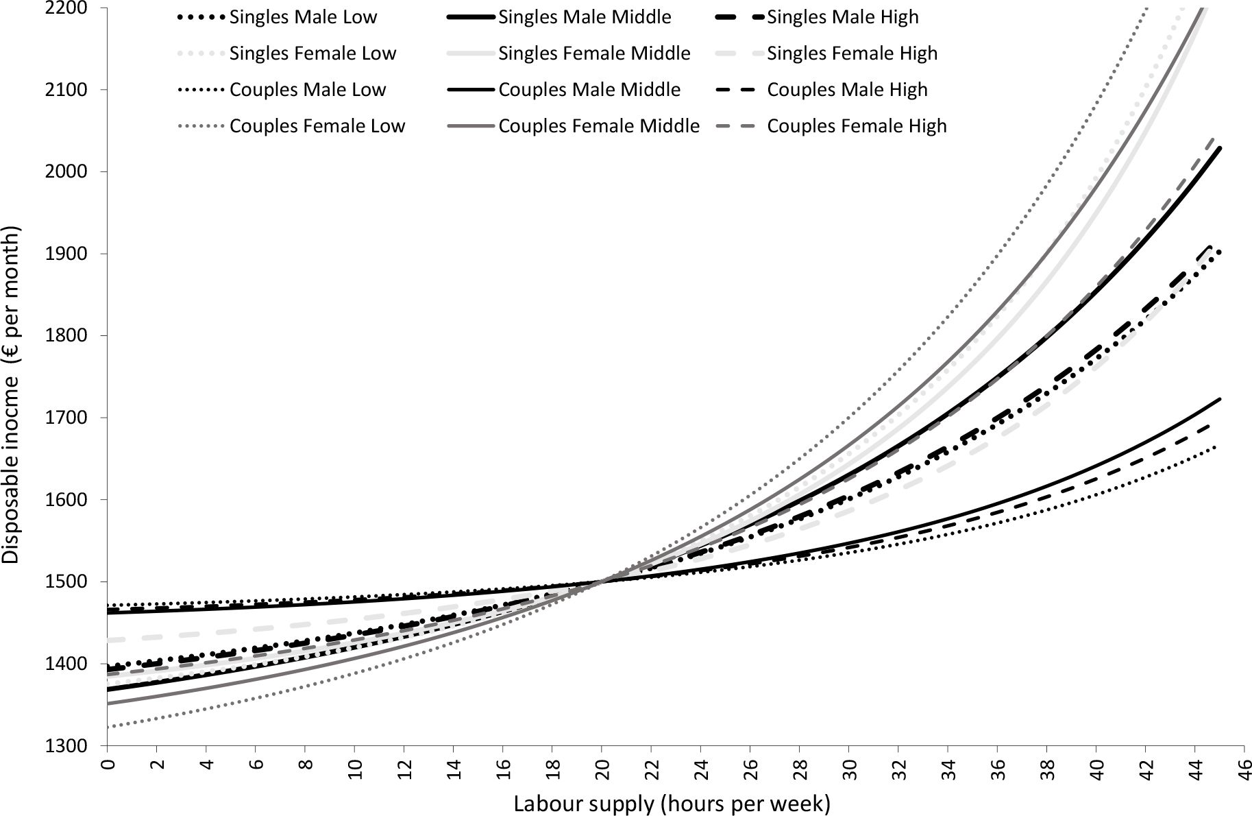
We illustrate this in Figure 2 for the education level. For males, both in couples (thin black curves in Figure 2), and as singles (fat black curves in Figure 2), the effect of education is non–monotonous. Both highly and lowly educated (dashed, respectively dotted curves) men have less intense preference for leisure relative to consumption, as compared to their fellows with a middle education level (full lines). This effect is more outspoken, but much less precisely estimated, in the case of singles. Higher educated females have less intense preferences for leisure relative to consumption, both when living in couples (dark grey curves) or as a single (light grey curves).

Impact of education level on steepness of indifference curves.
5.2 Opportunities
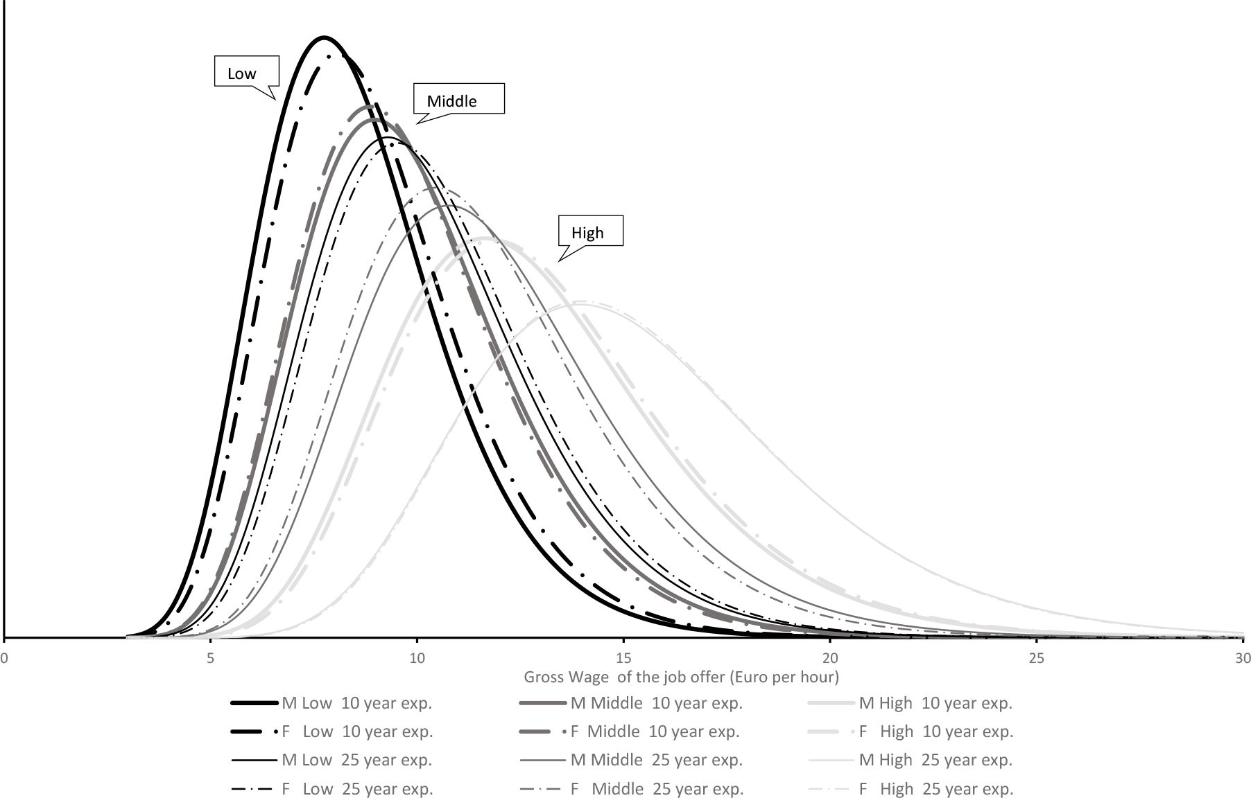
Figure 3 represents the estimation of the wage offer distributions. The dotted lines apply to females, the full lines to males. The sex differences are small, as compared to the impact of the other covariates, and not always in the disadvantage of females. The latter is the case for persons with a middle education level.

Estimated wage offer distributions and education.
Higher education shifts the wage offer distribution to the right: compare the fat black, grey, and light grey curves for the distributions at low experience age (10 years), and the thin black, grey, and light grey curves for the impact of education at high experience age (25 years). Potential experience also shifts the wage offer distribution to the right: compare fat and thin lines of the same color. However, when potential experience would exceed the level of 37 years, for males, and 32 years, for females, the wage offer distribution would start shifting to the left again. For experience levels below these bounds, higher education, which implies less potential experience, has therefore two countervailing effects on the wage distribution. The net effect is usually positive, that is a shift of the wage offer distribution to the right. Whether this would also results into an increased acceptance of jobs, depends on income and substitution effects (in preferences), and cannot be fixed apriori.
Notice that this is a wage offer distribution. Simulated and observed wages of accepted jobs are discussed in Section 6.
Figure 4 represents the distribution of offered labour time regimes.17 Again, these are not actual labour time regimes nor those chosen according to the model. The most salient observation is that this distribution is different for males and females, the latter receiving more part time, and less full time job offers.

Estimated distribution of offered labour time regimes.
Figure 5 reports the impact of education on the intensity of suitable job offers (the q–function).18 As the type specific unemployment rate varies with education level (and age) we report the joint effect of both. More specifically, for each age class we report the intensity of suitable job offers of males (black bars), respectively females (grey bars) of a lowly (dotted bar), highly educated persons (dashed bar), and those with middle education level (fully coloured bars).
Considered per se the education level has a positive effect on the availability of suitable job offers, though the effect of high versus middle education is small for males.
From Table 2 it can be seen that the type specific unemployment rate is decreasing in the education level. Now, for males, a higher type specific unemployment rate increases the intensity of suitable job offers. As a consequence, the already small positive effect of education is slightly attenuated, leading ultimately to a net negative effect of high as compared to middle education level for the middle age classes. For females on the other hand the net effect of high education is outspokenly positive, as both the effect of the lower unemployment rate with education and education per se, push into the same direction.
Notice that Figure 5 also reveals that the availability of suitable job offers is decreasing slightly with age for males, while we don’t see a similar decline for females.
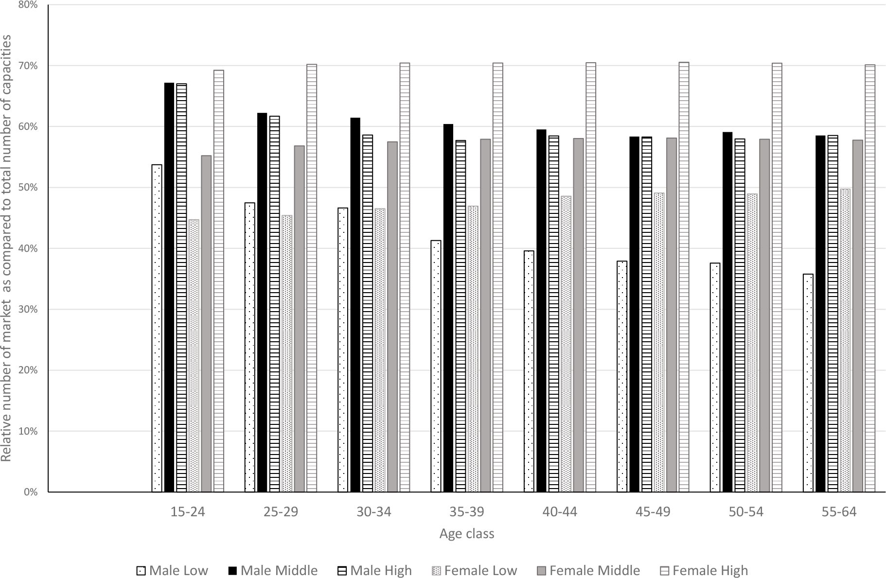

Job offer intensity in function of education and age specific unemployment rate.
6. Fit and behavioural response
6.1 Fit
We now evaluate the fit of the estimated model.
1. Couples
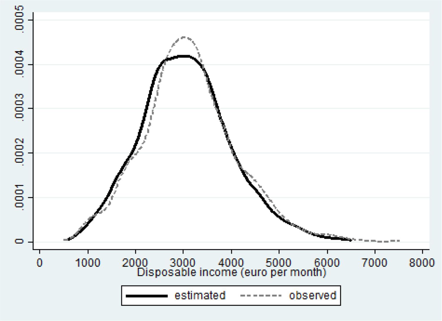
The mean estimated consumption within couples is 3070 € per month. Compare that with the observed mean of 3143 € per month reported in Table 1. The simulated distribution (black curve in Figure 6) slightly overestimates the number households with lower incomes, at the expense of those with modal disposable incomes (compare the black curve with the observed values represented by the gray dashed one).
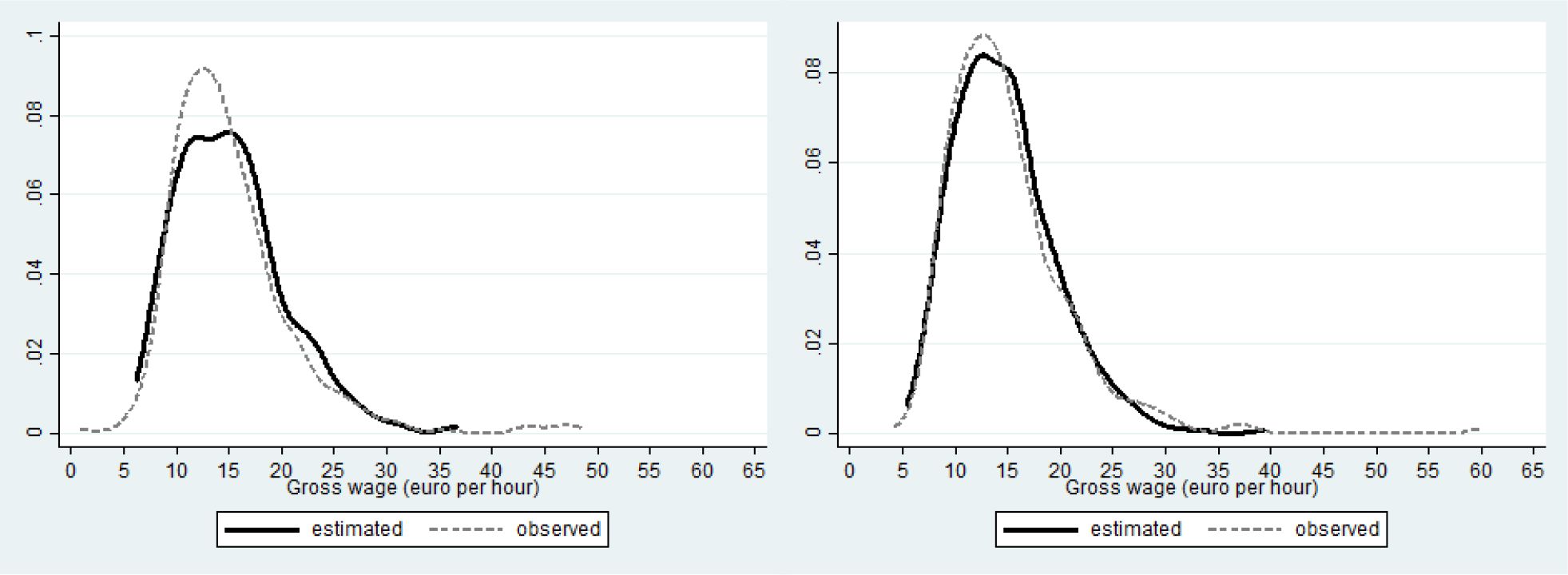
The fit of the (conditional) distribution of female wages is good (RhS panel of Figure 7): the black (simulated) and grey dashed (observed) curve almost coincide. The simulated wage distribution of the males (black line on the LhS panel of Figure 7) is more populated than the observed one (grey dashed line on the LhS panel of Figure 7) at lower and moderately high wages, at the expense of a smaller occurrence of modal and extremely high wages.
Fit disposable income for couples.
The number of non–participants in the labour market is overestimated. Compare thereto the full grey (observed) and unfilled black bordered (simulated) left most spike in both panels of Figure 8. Still, the number of cases in which none of both partners work, is underestimated. The estimated peaks reasonably well fit the observed values, except for the three quarter time jobs, the occurrence of which is underestimated by the model, both for male and female partners. The percentage of females having a full time job is also slightly overestimated by the model.

Fit wages males (left) and females (right) in couples.
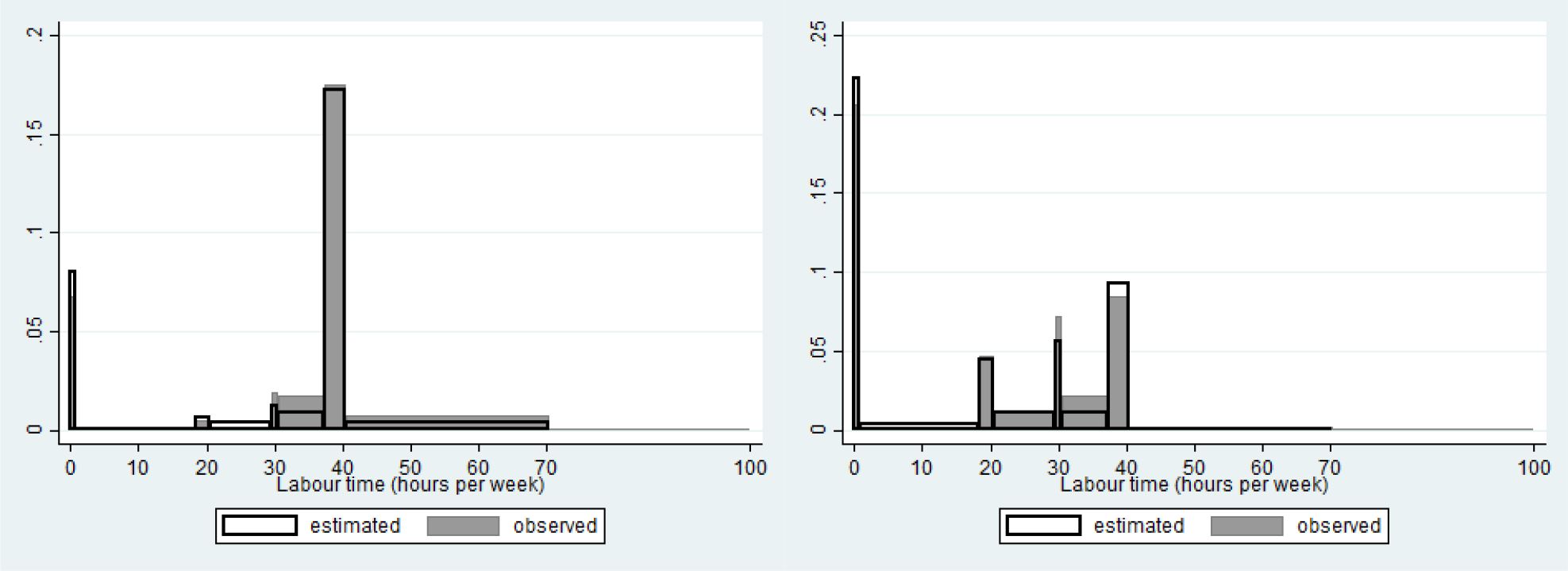
Fit labour time males (left) and females (right) in couples.
2. Singles
Figures 9–11 represent the fit of the model for singles. Consumption of single females is reasonably well approximated (rhs of Figure 9). Mean consumption of males is almost perfectly replicated by the estimates (1585 € per month fitted versus 1588 € per month observed), but the empirical distribution is somewhat less good approximated, with, amongst other things, an underestimation of the lower tail. The latter is also the case for the single females.
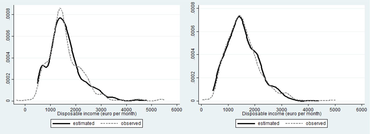
Fit disposable income single males (left) and single females (right).

Fit wages single males (left) and females (right).
Similarly, the wage distribution of single females (rhs of Figure 10) is better fitted than that of males (lhs of Figure 10).
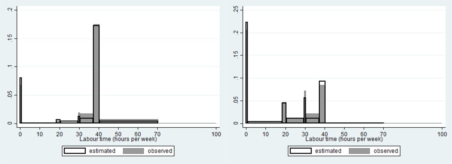
Labour market participation of single males (cf. lhs of Figure 11) is overestimated, while that of single females is almost perfectly fitted (rhs of Figure 11). The observed peak for half time jobs is underestimated for males, and that of three quarter time jobs is overestimated for both, males and females. The occurrence of full time jobs for males is overestimated. That of females underestimated.

Fit labour time regimes single males (left) and single females (right).
6.2 Elasticities
Table 4 reports the total reaction in terms of labour time and the effect on participation to the labour market (extensive margin), following a shift of the density of the males’, respectively females’, wage offer distribution to the right by 10% (augmenting the estimated location parameter with ln1.1). Additionally, we report intensive margins (effect on labour supply conditional on participating in the base line, inclusive of the labour market leavers). The variable ‘part in’ gives the percentage of entrants into the labour market, while ‘part out’ represents the percentage of leavers.
Aggregate wage elasticity of labour supply.
| Shift of female wage distribution | Shift of male wage distribution | |||||
|---|---|---|---|---|---|---|
| Couple | Single | Couple | Single | |||
| Female | Male | Female | Male | Female | Male | |
| Total elasticity | 0.6445 | -0.1734 | 0.6877 | -0.2014 | 0.3304 | 0.4569 |
| Intensive margin | 0.2162 | -0.2222 | 0.1257 | -0.2584 | 0.1365 | 0.0944 |
| Part in | 3.157% | 0.480% | 3.327% | 0.549% | 1.716% | 2.895% |
| Part out | 0.000% | 1.647% | 0.000% | 1.579% | 0.000% | 0.000% |
Compared to Marshallian elasticities in the literature estimated by static models using micro data, the total elasticity estimates produced here are rather large (Compare e.g. with the figures reported in Tables 6 and 7 of Keane, 2011). However, as far as these total elasticities include the extensive margin, and are calculated as the proportional change in total labour time for the whole sub-sample, these need to be compared with macro elasticities, which are usually much larger, even as compared to the figures obtained here.19 Still, it should be stressed that the figures reported here are conceptually of a different nature, in that actually obtained wages in the present model are the result of choosing the most attractive job offer according to the persons’ preferences. Therefore, a reaction to an exogenous change in that wage cannot be conceived of in the framework we used. What was, alternatively, done, is to shift the entire distribution of the wages included in the job offers, to the right. This cannot be considered the same as a change in an exogenously given wage. As the ruro model incorporates frictions due to restrictions in the labour market opportunities an agent faces, this might account for the lower values of the elasticities reported here, compared to values obtained for macro figures.
7. Education and labour market participation
In the present section we present a simulation exercise to assess the full effect of changes in education level on labour market participation and labour supply.
As our sample is not representative for the Belgian population at working age due to selecting only persons available for the labour market, currently not self-employed, we first produced a baseline in which we simulated the education level in accordance with the 2007 distribution, as produced by the Belgian dynamic microsimulation model midas (Federal Planning Bureau).20 More specifically, we replaced the currently observed education level for each individual in our sample with a randomly assigned education level based on the population figures for the age and gender specific education levels for this baseline (represented in the ‘baseline’ columns of Table 5).21 The potential experience and type specific unemployment rate were accordingly adapted. Then, we simulated labour market choices with these new data. Table 6 contains the participation rate (part) and average length of the work week h (including non–participants), by gender and age class, resulting from this exercise.
A similar procedure is then followed for the counterfactual scenario on education as obtained from the implementation in the MiDAS-model (see the ‘counterfactual’ columns of Table 5).
Notice that across all age classes, except the youngest, the number of females with higher education in the baseline exceeds that of males by five to ten percentage points. In the counterfactual scenario, the male education distribution is then modelled as approaching that of the females. The distribution of the educational attainment level is thus more or less equal for males and females in the ‘counterfactual’ columns.
Accordingly, we can learn from Table 6 that the overall effect of changing education levels over time is mainly concentrated among the men. More specifically, labour market participation of single males between 30 and 45 years old increases by 1.5 to over 7 percentage points. The mean number of hours worked per week for the same categories increases with half an hour to more than four hours. Female labour market participation and labour supply are not fundamentally affected in the alternative situation, as female education in the counterfactual does not differ much from that in the baseline. If anything, female labour market participation and labour time decrease slightly in the alternative scenario.
Education level distribution by age and sex.
| Education level | Low | Middle | High | |||
|---|---|---|---|---|---|---|
| Scenario | baseline | counterfactual | baseline | counterfactual | baseline | counterfactual |
| Age | males | |||||
| 15 – 25 | 21.20% | 20.10% | 40.15% | 39.90% | 38.65% | 39.99% |
| 26 – 30 | 27.42% | 19.84% | 41.27% | 40.00% | 31.31% | 40.16% |
| 31 – 35 | 27.27% | 19.44% | 40.41% | 40.13% | 32.32% | 40.43% |
| 36 – 40 | 27.66% | 20.47% | 40.22% | 39.75% | 32.11% | 39.78% |
| 41 – 45 | 26.87% | 19.80% | 39.22% | 40.24% | 33.92% | 39.96% |
| 46 – 50 | 26.62% | 20.33% | 39.68% | 39.97% | 33.71% | 39.70% |
| 51 – 55 | 26.12% | 20.50% | 38.15% | 39.84% | 35.73% | 39.67% |
| 56 – 60 | 25.35% | 20.15% | 38.79% | 39.95% | 35.86% | 39.90% |
| 61 – 65 | 24.15% | 19.96% | 38.66% | 39.70% | 37.18% | 40.33% |
| all | 27.27% | 20.90% | 41.54% | 41.42% | 31.19% | 37.68% |
| females | ||||||
| 15 – 25 | 20.36% | 20.21% | 40.23% | 40.12% | 39.41% | 39.68% |
| 26 – 30 | 20.22% | 19.51% | 39.77% | 40.38% | 40.01% | 40.11% |
| 31 – 35 | 18.71% | 20.26% | 38.09% | 40.12% | 43.20% | 39.62% |
| 36 – 40 | 19.77% | 19.31% | 38.35% | 39.69% | 41.89% | 41.00% |
| 41 – 45 | 19.61% | 20.14% | 38.03% | 39.68% | 42.36% | 40.19% |
| 46 – 50 | 19.35% | 20.46% | 38.27% | 39.58% | 42.38% | 39.96% |
| 51 – 55 | 19.14% | 20.12% | 38.03% | 38.80% | 42.83% | 41.08% |
| 56 – 60 | 20.03% | 19.33% | 38.73% | 40.48% | 41.24% | 40.19% |
| 61 – 65 | 19.46% | 20.11% | 39.01% | 39.80% | 41.53% | 40.09% |
| all | 20.52% | 20.79% | 40.26% | 41.17% | 39.22% | 38.04% |
-
Source: midas implemented scenarios for baseline coinciding with 2007 and counterfactual aiming at a catch-up of female’s higher education level than males’ in the baseline, by 2050.
All in all, the model predicts that expected shifts in the education level will not have a very large impact on labour market participation.
Participation and mean labour time by age class in baseline and counterfactual.
| Age | 15 – 25 | 26 – 30 | 31 – 35 | 36 – 40 | 41 – 45 | 46 – 50 | 51 – 55 | 56 – 60 | 61 – 65 | all |
|---|---|---|---|---|---|---|---|---|---|---|
| Couples: males | ||||||||||
| n obs | 68 | 182 | 247 | 290 | 243 | 132 | 148 | 90 | 16 | 1457 |
| part baseline | 89.7% | 90.1% | 88.7% | 94.1% | 92.2% | 94.8% | 93.2% | 74.4% | 87.5% | 90.9% |
| part counterf. | 89.7% | 92.3% | 89.1% | 94.5% | 93.4% | 96.0% | 93.2% | 80.0% | 87.5% | 92.0% |
| h baseline | 33.4 | 34.3 | 35.9 | 38.8 | 37.2 | 38.3 | 37.4 | 28.2 | 35.8 | 36.4 |
| h counterf. | 33.4 | 35.1 | 36.2 | 39.0 | 37.6 | 38.6 | 37.2 | 30.2 | 35.8 | 36.7 |
| Couples: females | ||||||||||
| n obs | 124 | 241 | 264 | 260 | 230 | 172 | 99 | 58 | 9 | 1457 |
| part baseline | 74.2% | 78.8% | 73.5% | 78.8% | 82.2% | 80.8% | 73.7% | 72.4% | 55.6% | 77.5% |
| part counterf. | 73.4% | 77.2% | 73.5% | 78.1% | 81.3% | 80.2% | 75.8% | 69.0% | 55.6% | 76.8% |
| h baseline | 24.3 | 25.4 | 23.2 | 24.7 | 26.0 | 24.9 | 20.9 | 22.7 | 18.1 | 24.4 |
| h counterf. | 24.2 | 24.7 | 23.0 | 24.4 | 25.6 | 24.3 | 21.6 | 22.1 | 18.1 | 24.0 |
| Singles: females | ||||||||||
| n obs | 43 | 59 | 83 | 97 | 89 | 82 | 55 | 51 | 12 | 571 |
| part baseline | 58.1% | 69.5% | 69.9% | 66.0% | 65.2% | 79.3% | 80.0% | 70.6% | 50.0% | 69.5% |
| part counterf. | 58.1% | 69.5% | 68.7% | 66.0% | 65.2% | 78.0% | 80.0% | 70.6% | 50.0% | 69.2% |
| h baseline | 18.4 | 23.6 | 27.1 | 23.6 | 21.9 | 27.1 | 24.8 | 21.8 | 14.3 | 23.7 |
| h counterf. | 18.4 | 23.6 | 26.6 | 23.6 | 21.9 | 26.8 | 24.8 | 21.8 | 14.3 | 23.6 |
| Singles: males | ||||||||||
| n obs | 46 | 60 | 67 | 68 | 54 | 65 | 46 | 33 | 10 | 449 |
| part baseline | 80.4% | 88.3% | 91.0% | 77.9% | 85.2% | 87.7% | 67.4% | 72.7% | 50.0% | 80.6% |
| part counterf. | 80.4% | 83.3% | 92.5% | 85.3% | 87.0% | 87.7% | 69.6% | 72.7% | 60.0% | 83.1% |
| h baseline | 31.5 | 30.3 | 34.6 | 30.0 | 32.8 | 33.2 | 23.3 | 25.2 | 18.5 | 30.4 |
| h counterf. | 31.5 | 32.1 | 35.1 | 34.2 | 33.6 | 33.3 | 24.7 | 25.2 | 22.1 | 31.7 |
Impact of education through preferences and opportunities.
| Couple | Single | |||
|---|---|---|---|---|
| Males | Females | Males | Females | |
| n obs | 1457 | 1457 | 449 | 571 |
| part base | 90.87% | 77.48% | 80.62% | 69.53% |
| part alt pref | 90.94% | 77.62% | 81.51% | 69.53% |
| part alt opp | 91.90% | 76.94% | 82.85% | 69.35% |
| part counterf. | 91.97% | 76.80% | 83.07% | 69.17% |
| h base | 36.35 | 24.35 | 30.37 | 23.72 |
| h alt pref | 36.27 | 24.32 | 30.82 | 23.72 |
| h alt opp | 36.78 | 24.12 | 31.38 | 23.67 |
| h counterf. | 36.73 | 24.04 | 31.67 | 23.60 |
In Table 7 we give an idea of the relative contribution of preferences and opportunities to the explanation of this moderate shift. Recall from Figure 2 that males with lower and higher education level have more intense preferences for leisure, than those with middle education levels, while the intensity of preferences for leisure of females is monotonically decreasing in the education level. On the other hand, the intensity of suitable job offers is increasing with education level, but there is a countervailing effect of higher education on the wage distribution as potential experience will decrease. In Table 7 the figures for participation (part) and labour time (h) labelled by ‘base’ and ‘counterf.’ repeat the population labour participation and average labour time (hours per week) for the corresponding scenarios from the last column of Table 6. The rows labelled by ‘alt pref’ use the education level in the preferences according to the alternative scenario (a shift from low to high for men, a small increase of middle at the expense of high for females, see Table 5), but keep the wage offer distribution and job offer intensity corresponding to the education levels in the baseline. Except for single males, participation figures are hardly affected by this change in education level through preferences. Participation of single males increases with almost one percentage point and they work on average half an hour longer. This cannot easily be explained by the indifference curves (as the high and low educated males have almost identical indifference curves), but must be the consequence of the interaction of wage and income effects which might be different at different utility levels.
The rows with label ‘alt opp’ correspond to figures obtained by the wage offer distribution and job offer intensity with education levels as in the alternative scenario, while keeping the education profile of the baseline along the preference side of the model. Participation and labour time of females decreases slightly, which means that the increased potential experience gain due to lower education does not counterbalance the effect of lower intensity of job offers. Participation of men in couples increases with one percentage point and that of single males with more than two percentage points. Average labour time of the latter is one hour higher, but increases only half an hour for males in couples. Also for males, the lower potential experience age due to higher education does not seem to counterbalance the effect of higher job offer intensity.
We conclude that the already small change in labour market participation due to expected changes in education level, run predominantly through the channel of opportunities rather than through preferences.
8. Conclusion
In the present paper we have explained how to estimate a ruro model. Next, we illustrated how the model can be used in simulation exercises.
We think the ruro framework might prove useful in modelling behavioural reactions to tax-benefit reforms as assessed by micro-simulation models. Moreover it provides a tool to throw some light on the extent to which the impact of such reforms runs through preferences, or rather through the channel of modifying opportunities. The latter is not only a question of modifications in the budget set, but also the availability of jobs in accordance with a person’s capacities comes into play. As this distinction is at the heart of some policy debates, such as the extent to which a tax shift from labour to consumption might create more jobs, we feel the approach presented here is also relevant from a policy point of view.
Of course there are some limitations too. The model is essentially static. And it does not provide a complete equilibrium framework. It is not a matching model in which job offers are matched (or not) to suitable candidates. Frictions on the labour market are taken as given. Within this containment however, it is possible to make a distinction between the impact of measures that runs through preferences, and the part that can be attributed to opportunities.
Footnotes
1.
Recent overviews of the model and its applications are provided by Aaberge and Colombino (2014), and Dagsvik, Jia, Kornstad, and Thoresen (2014).
2.
Some contributions do allow for unobserved wage heterogeneity, see e.g. Van Soest, Das and Gong (2002), Löffler et al. (2013), and the second model discussed in Dagsvik and Jia (2016). Van Soest (1995) already incorporated the problem of imperfect observation of wages for non–participants in the extended version of his model. Besides, there is an earlier literature accounting for the fact that wages are non–linear in hours (See for example Moffitt, 1984). However, none of these treats wages as an object of job choice behaviour. In our model, there is no unobserved wage heterogeneity, neither measurement error in wages. The wages in our model are, as in the first class of models of Dagsvik and Jia (2016), part of the job offers available to an individual.
3.
Statistics on Income and Living Conditions (silc) is a survey held yearly in EU-member states and some other countries under supervision of eurostat. Permission to use eu-silc data for Belgium was obtained in the framework of the euromod-project. More in formation on eu-silc can be found on http://ec.europa.eu/eurostat/web/microdata/european-union-statistics-on-income-and-living-conditions. See Section 4 for more information on the data we used from eu-silc.
4.
Currently males’ educational attainment level is lagging behind that of females.
5.
We include the gross wage, and the number of hours worked as separate arguments in that function, as some aspects of the tax system, such as the Belgian work bonus, may depend on the wage, rather than on labour income, wh. We are however aware that this might cause problems for the non–parametric identification of the ruro model.
6.
The word ‘activity’ will be used here in a broad sense, including occupations which are not very ‘active’ such as sleeping and day dreaming. A certain type of agency or control is however presumed, since otherwise it would be difficult to talk about choice behaviour.
7.
In Appendix A1, we provide a brief introduction to the type of stochastic process that describes the degree to which job offers and non–market alternatives become available to an individual, and which is known as an inhomogeneous spatial Poisson process.
8.
Job offer arrivals depend on personal capacities and skills which are subdivided in those apt to execute formal jobs, and those suited for performing leisure activities. Next there may be personal characteristics on the basis of which discrimination in job offers by employers might take place. As indicated before, we omit the impact of these conditioning variables for the sake of notational simplicity.
9.
As mentioned before, a ‘job offer’ is a short hand for ‘an alternative containing at least one job offer’.
10.
In general, the class of Fréchet distributions is defined as: , where μ is a location parameter, σ a scale parameter, and α is a shape parameter.
11.
Ideally one would use the number of vacancies for suitable jobs for certain identifiable groups of persons in the population, but, such information is not really observable.
12.
More details are provided in Section 5.1.
13.
The issue of sampling choice sets for estimating the ruro model is discussed more in detail in McFadden (1978), Ben-Akiva and Lerman (1985), Aaberge, Colombino and Wennemo (2009), Train (2009), and Lemp and Kockelman (2012).
14.
The exact figures are for males, and the corresponding numbers for females are .246, 2.63, and .297.
15.
Version F5.5 was used. For more information about euromod, see Sutherland and Figari (2013) and http://www.iser.essex.ac.uk/euromod.
16.
For each draw (ws, hs), the disposable income f (ws, hs; xf) is again obtain from the microsimulation model euromod.
17.
Admittedly, this part of the model is not non–parametrically identified (see Section 3.2). So, if one feels more for explaining this peak pattern by preferences, we cannot tell this to be wrong on purely empirical grounds.
18.
We actually report values for q/ (1 + q). In this way the results are normalised to lie between zero and one.
19.
On the controversy about micro versus macro estimates, see amongst others Chetty et al. (2011), Chetty (2012), Fiorito and Zanella (2012), Keane and Rogerson (2012), Jantti et al. (2015), and the references therein.
20.
As midas runs on administrative data that do not include information on education levels, these were imputed, and some basic scenarios were developed to assess their evolution in the future, as new, future generations enter the model. More information on midas can be found in Dekkers et al. (2009).
21.
Education levels were assigned on the basis of a comparison of a random draw from the [0, 1]–uniform distribution for each case, with the cumulative distribution of education levels in the corresponding gender and age class of the individual.
A1. Poisson processes
Originally, a Poisson process is a stochastic process describing the probability of the number of occurrences of a particular event during a certain time spell. More specifically, a Poisson process assumes that the distribution of the time between each pair of consecutive events is independent from the moment at which the first of these two events occurred, or from any other event in the past, and that these inter-arrival times are exponentially distributed with parameter λ. This parameter λ measures the intensity with which such events occur. Under these assumptions, the probability that a certain event occurs n times within a given unit of time, with n £ {0,1,2...}, equals:
where N (t) is the number of events that occurred in total after t units of time.
Equation (a.1) is a Poisson distribution with intensity parameter λ. More generally, for a Poisson process, it holds that the number of events occurring within an interval of length τ is Poisson distributed with parameter λτ:
In this standard Poisson process, λ · τ is the expected number of events to occur within a time interval of length τ.
A Poisson process is inhomogeneous if the intensity parameter depends on the moment of measurement, λ (t) say. In that case, the probability that n events occur within a time interval [t, t + τ], equals:
where , is the expected number of times the event occurs in the interval [t, t + τ].
A Poisson process can also be spatial. Let an event be described as a point in an m–dimensional space. A spatial Poisson process determines the probability that n events occur within a subset of the m-dimensional space. Let, for example, ℬ be a subset of ℝm with volume .
Furthermore, let N (ℬ) be the number of events occurring in ℬ. If the occurrence of such events obeys a spatial Poisson process with intensity parameter λ, then the probability that there occur n events in ℬ, follows a Poisson distribution :
More generally, for such a spatial Poisson process, the number of events to occur within a set ℬ with volume ρ (ℬ) not necessarily equal to one, is Poisson distributed with parameter λρ (ℬ):
Again, λρ (ℬ) is the expected number of events to occur in set ℬ.
Such a spatial Poisson process is said to be inhomogeneous if the intensity of occurrence depends on the points x £ ℝm. To describe that process, assume that there exists a measure ρ defined on (measurable) subsets of the space ℝm, and let the intensity function λ (x) be integrable with respect to that measure. The probability that there occur n events in a measurable subset ℬ of ℝm, is then:
where , is equal to the expected number of events in the set ℬ.
Job offers and the availability of non–market activities each are described by an inhomogeneous spatial Poison process in ruro models. These processes are independent.
A2. Likelihood: the case of couples
Assume that both partners have identical tastes specified over household consumption, each of the partners’ leisure time, and other attributes associated with the activities the partners executed. From these assumptions, a utility function, say Ψ, can be derived in terms of both spouses’ wages and hours of labour time, (w1, h1, w2, h2). If one assumes that each partner’s process of job offer arrivals and availability of non–market alternatives is independent of that of the other, the following expressions for the likelihood are obtained, for the cases respectively that both partners, only one of them, or none of both will accept a job offer:
with
and are the relative intensity of job offers, the wage offer density, and the labour time density of partner j (j = 1, 2). For couples, a non–market alternative is an alternative in which none of both partners is engaged in the formal labour market.
A3. Coefficient estimates
Preferences couples.
| Log likelihood | −8482.1758 | ||
|---|---|---|---|
| Description | Estimate | Standard Error | t-value |
| 1.a) Consumption & leisure interaction M&F | |||
| Consumption Couples exponent | 0.610 | 0.051 | 11.96 |
| Consumption Couples constant | 4.873 | 0.310 | 15.70 |
| Leisure interaction M&F.in couples | 0.206 | 0.077 | 2.69 |
| Consumption single M exponent | 0.292 | 0.123 | 2.38 |
| Consumption single M constant | 4.740 | 0.395 | 12.00 |
| Consumption single F exponent | 0.049 | 0.149 | 0.33 |
| Consumption single F constant | 4.181 | 0.338 | 12.36 |
| 1.b) Leisure coefficients males in couples | |||
| Leisure M in couples exponent | −8.351 | 0.663 | −12.59 |
| Leisure M in couples constant | 20.959 | 7.880 | 2.66 |
| Leisure M in couples ln(age) | −11.339 | 4.321 | −2.62 |
| Leisure M in couples ln(age)2 | 1.591 | 0.601 | 2.65 |
| Leisure M in couples ch03 | 0.007 | 0.059 | 0.12 |
| Leisure M in couples ch36 | 0.078 | 0.063 | 1.23 |
| Leisure M in couples ch69 | −0.009 | 0.058 | −0.15 |
| Leisure M in couples dum region Walloona | 0.132 | 0.068 | 1.94 |
| Leisure M in couples dum region Brusselsa | 0.168 | 0.112 | 1.49 |
| Leisure M in couples dum education LOWb | −0.174 | 0.085 | −2.05 |
| Leisure M in couples dum education HIGHb | −0.078 | 0.060 | −1.31 |
| 1.c) Leisure coefficients females in couples | |||
| Leisure F in couples exponent | −6.995 | 0.502 | −13.93 |
| Leisure F in couples constant | 32.068 | 14.700 | 2.18 |
| Leisure F in couples ln(age) | −18.521 | 8.368 | −2.21 |
| Leisure F in couples ln(age)2 | 2.879 | 1.197 | 2.40 |
| Leisure F in couples ch03 | 0.550 | 0.179 | 3.08 |
| Leisure F in couples ch36 | 0.533 | 0.187 | 2.84 |
| Leisure F in couples ch69 | 0.426 | 0.191 | 2.23 |
| Leisure F in couples dum region Walloona | 0.302 | 0.173 | 1.74 |
| Leisure F in couples dum region Brusselsa | 0.062 | 0.247 | 0.25 |
| Leisure F in couples dum education LOWb | 0.612 | 0.331 | 1.85 |
| Leisure F in couples dum education HIGHb | −0.753 | 0.183 | −4.10 |
-
a
Flanders region is reference category.
-
b
Middle education level is reference category.
Preferences singles.
| Description | Estimate | Standard Error | t-value |
|---|---|---|---|
| 1.d) Leisure coefficients single males | |||
| Leisure single M exponent | −5.444 | 1.002 | −5.43 |
| Leisure single M constant | 36.394 | 23.737 | 1.53 |
| Leisure single M ln(age) | −20.375 | 13.239 | −1.54 |
| Leisure single M ln(age)2 | 3.024 | 1.865 | 1.62 |
| Leisure single M ch36 | −0.457 | 1.112 | −0.41 |
| Leisure single M ch69 | −1.135 | 0.698 | −1.63 |
| Leisure single M dum region Walloona | 0.951 | 0.425 | 2.24 |
| Leisure single M dum region Brusselsa | 0.262 | 0.372 | 0.70 |
| Leisure single M dum education LOWb | −0.581 | 0.387 | −1.50 |
| Leisure single M dum education HIGHb | −0.502 | 0.335 | −1.50 |
| 1.e) Leisure coefficients single females | |||
| Leisure single F exponent | −7.688 | 0.977 | −7.87 |
| Leisure single F constant | 62.678 | 23.311 | 2.69 |
| Leisure single F ln(age) | −34.609 | 12.929 | −2.68 |
| Leisure single F ln(age)2 | 4.876 | 1.809 | 2.70 |
| Leisure single F ch03 | 0.838 | 0.502 | 1.67 |
| Leisure single F ch36 | 0.128 | 0.239 | 0.54 |
| Leisure single F ch69 | −0.141 | 0.196 | −0.72 |
| Leisure single F dum region Walloona | 0.212 | 0.199 | 1.06 |
| Leisure single F dum region Brusselsa | −0.258 | 0.188 | −1.37 |
| Leisure single F dum education LOWb | 0.133 | 0.326 | 0.41 |
| Leisure single F dum education HIGHb | −0.616 | 0.217 | −2.84 |
-
a
Flanders region is reference category;
-
b
Middle education level is reference category.
Opportunities, relative intensity of market alternatives, peaks hours, and wage offer distribution.
| Description | Estimate | Standard Error | t-value |
|---|---|---|---|
| 2.a) Estimated coefficients opportunities & peaks males | |||
| Opportunity M constant | −4.488 | 0.247 | −18.19 |
| Opportunity M unemployment rate | 0.338 | 0.226 | 1.50 |
| Opportunity M dummy region Walloona | −0.547 | 0.223 | −2.45 |
| Opportunity M dummy region Brusselsa | −1.215 | 0.285 | −4.27 |
| Opportunity M dummy LOW educationb | −0.987 | 0.277 | −3.56 |
| Opportunity M dummy HIGH educationb | 0.049 | 0.265 | 0.19 |
| Peaks M <18.5,20.5> interval | 0.643 | 0.229 | 2.81 |
| Peaks M <29.5,30.5> interval | 0.862 | 0.189 | 4.55 |
| Peaks M <37.5,40.5> interval | 2.690 | 0.060 | 45.17 |
| 2.b) Estimated coefficients opportunities & peaks females | |||
| Opportunity F constant | −4.300 | 0.185 | −23.19 |
| Opportunity F unemployment rate | −0.072 | 0.124 | −0.58 |
| Opportunity F dummy region Walloona | −0.394 | 0.157 | −2.51 |
| Opportunity F dummy region Brusselsa | −0.783 | 0.219 | −3.58 |
| Opportunity F dummy LOW educationb | −0.339 | 0.217 | −1.56 |
| Opportunity F dummy HIGH educationb | 0.522 | 0.195 | 2.68 |
| Peaks F <18.5,20.5> interval | 1.636 | 0.100 | 16.42 |
| Peaks F <29.5,30.5> interval | 1.804 | 0.108 | 16.69 |
| Peaks F <37.5,40.5> interval | 2.206 | 0.070 | 31.36 |
| 3. Estimated coefficients wage equations | |||
| 3.a) Wage equation males | |||
| Wage M σ | 0.264 | 0.004 | 60.63 |
| Wage M constant | 2.066 | 0.029 | 72.00 |
| Wage M potential experience | 2.297 | 0.244 | 9.41 |
| Wage M potential experience2 | −3.110 | 0.545 | −5.71 |
| Wage M LOW educationb | −0.147 | 0.019 | −7.79 |
| Wage M HIGH educationb | 0.260 | 0.015 | 17.39 |
| 3.b) Wage equation females | |||
| Wage F σ | 0.261 | 0.004 | 59.05 |
| Wage F constant | 2.043 | 0.026 | 77.61 |
| Wage F potential experience | 2.457 | 0.239 | 10.30 |
| Wage F potential experience2 | −3.869 | 0.592 | −6.54 |
| Wage F LOW educationb | −0.095 | 0.023 | −4.08 |
| Wage F HIGH educationb | 0.291 | 0.016 | 18.61 |
-
a
Flanders region is reference category;
-
b
Middle education level is reference category.
References
-
1
Labour supply modelsIn: C O’Donoghue, editors. Handbook of Microsimulation Modelling, Contributions to economic Analysis, 293. Bingley: Emerald Group Publishing Ltd.. pp. 167–221.
-
2
Labour supply in Italy: an empirical analysis of joint decisions, with taxes and quantity constraintsJournal of Applied Econometrics 14:403–422.
-
3
Evaluating alternative representations of the choice sets in models of labour supplyJournal of Economic Surveys 23:586–612.
-
4
Labor supply responses and welfare effects of tax re-formsScandinavian Journal of Economics 97:635–659.
-
5
Labor supply preferences, hours constraints, and hours-wage trade-offsJournal of Labor Economics 6:254–276.
-
6
Labor supply, hours constraints, and job mobilityJournal of Human Resources 27:256–278.
- 7
- 8
- 9
-
10
Job search, hours restrictions, and desired hours of workJournal of Labor Economics 26:137–179.
-
11
Bounds on elasticities with optimization frictions: a synthesis of micro and macro evidence on labor supplyEconometrica 80:969–1018.
-
12
Are micro and macro labor supply elasticities consistent? A review of evidence on the intensive and extensive marginsAmerican Economic Review 101:471–475.
-
13
Discrete and continuous choice, max-stable processes, and independence from irrelevant attributesEconometrica 62:1179–1205.
-
14
Justification of functional form assumptions in structural models: a correctionTheory and Decision 75:79–83.
-
15
Justification of functional form assumptions in structural models: applications and testing of qualitative measurement axiomsTheory and Decision 70:215–254.
-
16
Labor supply as a choice among latent jobs: unobserved heterogeneity and identificationJournal of Applied Econometrics 31:487–506.
-
17
Theoretical and practical arguments for modeling labor supply as a choice among latent jobsJournal of Economic Surveys 28:134–151.
-
18
Simulating labor supply behaviour when workers have preferences over job opportunities and face non–linear budget constraints. Discussion paper no. 01/2006child, Torino, Italy: Centre for Household, Income, Labour and Demographic Economics.
-
19
Evaluation of tax reforms when workers have preferences over job attributes and face latent choice restrictions. Discussion paper no. 13/2007child, Torino, Italy: Centre for Household, Income, Labour and Demographic Economics.
-
20
Labour supply with non–convex budget sets, hours restriction and non–pecuniary job attributes. Discussion Paper No 76Central Bureau of Statistics Norway.
-
21
Analyzing labor supply behavior with latent job opportunity sets and institutional choice constraints. Discussion Paper No 344Statistics Norway, Research Department.
-
22
Sectoral labour supply, choice restrictions and functional form. Discussion paper no. 388Statistics Norway, Research Department.
-
23
Sectoral labour supply, choice restrictions and functional formJournal of Applied Econometrics 21:803–826.
-
24
What are the consequences of the European AWG-projections on the adequacy of pensions? An application of the dynamic micro simulation model midas for Belgium, Germany and Italy. ENEPRI Research Report No. 65, AIM WP4Centre for European Policy Studies.
- 25
-
26
The anatomy of the aggregate labor supply elasticitiesReview of Economic Dynamics 15:171–187.
-
27
Testing intertemporal substitution, implicit contracts, and hours restriction models of the labor market using micro dataAmerican Economic Review 92:905–927.
-
28
Taxes and labor supplyIn: AJ Auerbach, M Feldstein, editors. Handbook of Public Economics. Amsterdam: Elsevier Science Publishers B.V. (North-Holland). pp. 213–263.
-
29
Estimating labour supply elasticities based on cross-country micro data: A bridge between micro and macro estimates?Journal of Public Economics 127:87–99.
- 30
-
31
Micro and macro labor supply elasticities: a reassessment of conventional wisdomJournal of Economic Literature 50:464–476.
-
32
Strategic sampling for large choice sets in estimation and appli-cationTransportation Research Part A 46:602–613.
-
33
Structural labor supply models and wage exogeneity. iZA dp No.8281Forschungsinstitut zur Zukunft der Arbeit.
-
34
Individual Choice Behavior: A Theoretical Analysisrepr. 2005, Individual Choice Behavior: A Theoretical Analysis, Mineola (New York), Dover Publications Inc.
-
35
Conditional logit analysis of qualitative choice behaviorIn: P Zarembka, editors. Frontiers in Econometrics. New York: Academic Press. pp. 105–142.
-
36
Modelling the choice of residential locationIn: A Karlqvist, L Lundqvist, F Snickars, J Weibull, editors. Spatial Interaction Theory and Planning Models. Amsterdam: North-Holland. pp. 75–96.
-
37
The estimation of a joint wage-hours labor supply modelJournal of Labor Economics 2:550–566.
-
38
euromod: the European Union tax-benefit microsimulation modelInternational Journal of Microsimulation 6:4–26.
-
39
Discrete Choice Methods with Simulation (2nd ed)Cambridge: Cambridge University Press.
-
40
A simultaneous wage and labor supply model with hours restric-tionsJournal of Human Resources 26:393–423.
-
41
Structural models of family labor supply: a discrete choice approachThe Journal of Human Resources 30:63–88.
-
42
A structural labour supply model with flexible preferencesJournal of Econometrics 107:345–374.
-
43
Labor supply, income taxes, and hours restrictions in the Netherlands517–558, Kapteyn A, Journal of Human Resources, 25, 3, Special Issue on Taxation and Labor Supply in Industrial Countries.
Article and author information
Author details
Acknowledgements
We are grateful to Rolf Aaberge and Ugo Colombino for an introduction into and many discussions on the ruro model, to Tom Wennemo for technical assistance with the estimation program, to two anonymous referees and the editor of this journal, to Bart Cockx, John Dagsvik, Erik Schokkaert, Dirk Van de gaer, and to the members of the advisory board of the MiMBEL-project for their comments on earlier versions of this article. Pieter Vanleenhove, Toon Vanheukelom and Rembert De Blander prepared the data from eu-silc 2007, and used euromod version F5.5 to calculate net incomes for the choice sets. We acknowledge financial support from the BELSPO-project mimbel. The usual disclaimer applies.
Publication history
- Version of Record published: August 31, 2016 (version 1)
Copyright
© 2016, Capéau
This article is distributed under the terms of the Creative Commons Attribution License, which permits unrestricted use and redistribution provided that the original author and source are credited.