Intertemporal income in Ireland 1996–2011 – a spatial analysis

In this paper the distribution of disposable income will be examined in a spatial context. Disposable income is not homogenous across space therefore it will be influenced across place (Kilroy, 2009). There are structural differences between regions (Heshmati, 2004) such as local specific policies (Shankar & Shah, 2003), local labour markets and agglomeration effects (Rosenthal & Strange, 2001). There exists a spatial dimension to the income distribution which can impact positively or negatively. It should be the aim of policy to reduce this inequality in the distribution of income.

The literature on spatial distribution of income is vast and diverse. Studies have focused on income at a regional (O’Leary, 1999), national (Slesnick, 2001) and international scale (Caselli, 2005). Some of these studies have focused on the clustering of poor/rich regions (Dall’Erba, 2005). The effect of policy on reducing regional disparities has been covered (Becker et al., 2010). Different locations will therefore have different levels of income (Sommeiller, 2006).

The focus of this paper is intertemporal disposable income. We would expect the spatial distribution of disposable income to change due to factors such as migration between urban and rural areas. The pull factors of urban areas include higher wages (Fields, 1975), a perceived better quality of life, more career opportunities, furthering education and access to more services (Blomquist et al., 1988). The pull factors in rural areas include natural environments, lower living costs, lower congestion and a more attractive lifestyle (Roback, 1982). These are countered by push factors such as higher living costs, higher crime rates, traffic congestion and pollution in urban areas and low education and employment opportunities in rural areas. As a result of these factors, wages are typically higher in urban areas.

The economic climate and labour market situation in a particular region affects the income distribution. Job losses can have a significant effect on a region. Similarly regions may benefit from agglomeration economies (Rosenthal & Strange, 2004), such as the clustering of industries and expertise in an area (Marshall, 1920). By observing spatial distributions over time, we can observe and attempt to track the changes in the spatial distribution of income.

The period covered in this paper was an economically turbulent period in Irish history. The Celtic Tiger (1995–2006) was a period of strong economic growth largely due to FDI. Real GDP growth averaged 10% a year (Honohan & Walsh, 2002). This period saw significant growth in the CPI. In the period 1996–2002, CPI grew by 18%, from 2002–2006 by 11% and 2006–2011 by 6%. Overall the CPI increased in the period 1996–2011 by 31%. The property bubble (2001–2007) saw house prices increase rapidly due to a combination of factors including; Government policy, banks’ lending practices and media coverage (Donovan & Murphy, 2013). House prices more than quadrupled between 1995–2007 (Kanda, 2010). A combination of the global financial crisis and collapse of the property market caused Ireland to enter a deep recession with GDP decreasing by 8% in 2009 alone (Kanda, 2010). The so called “Great Recession” was felt more strongly in Ireland due to double shocks hitting at the same time (global financial crisis and collapse of property market). In the space of four years unemployment more than doubled (2007–4.7%, 2011–14.6%) and net government debt increased 8 fold (2007–10% of GDP, 2011–81% of GDP), primarily through bank bailouts. This is in contrast to the period 1994–2004 where growth in real GNP was over 6% on average. In the same period unemployment fell from 15% to under 5% (Barrett & McCarthy, 2007). Whelan (2013), give a nice overview of the macroeconomic background in Ireland over the period 1988–2013, which additionally notes the impact of austerity measures on incomes. With this story taking place this paper aims to examine the changing distribution of income over this interesting time period which includes years of extraordinary growth as well as large contractions of the economy.

One of the results of the crisis are the so called “ghost estates” (residential units unfinished or abandoned) (Kitchin et al., 2010). Census data 2011 shows that there was an oversupply of housing, with approximately 15% vacancy rates (SAPS, 2011). This problem is especially bad in the former upper Shannon Rural Renewal Scheme area, where a building tax incentive scheme existed between 1999 and 2008. The area now contains 18% of all “ghost estates” (Kitchin et al., 2014).

Much of the story around this period has focused on the national scale. Not much attention has been paid to whether different areas were affected more or less than others. The NSS (2002) was a key policy document which aimed towards achieving balanced regional development in Ireland. However there was a lack of commitment to the strategy which saw it viewed as a document offering advice to policymakers and planners (Meredith & Van Egeraat, 2013). Another issue was the selection of the “gateways” and “hubs”. There was disagreement over the selection of some cities and towns over others. It was seen as “winners” and “losers” type selection policy (Daly & Kitchin, 2013). The CEDRA report (CEDRA, 2013) detailed specific recommendations on how to improve rural areas. With this in mind it is important to note the political sensitivities around stating one place should be developed over another. Meredith and Faulkner (2014), examined the geography of the labour force in Ireland 1991–2011 but found little change in labour characteristics of areas over this period. This paper builds on this by examining changes in income over time.

In this paper we examine spatial characteristics at the electoral district (ED) level. There are 3,440 EDs in Ireland, with an average population of around 1,345 in each. In order to examine income at the ED level we will require appropriate data. A Spatial Microsimulation approach helps us in overcoming the lack of ED level income data in published Census data. The follow section outlines the Spatial Microsimulation process.

As mentioned previously the SMILE model contains survey and census data in simulating incomes. The survey data for the years 1996 & 2002 comes from the Living in Ireland (LII) Survey. LII forms the Irish component of the European Community Household Panel (ECHP). 3,174 households completed the survey in 1996. From 2001 a new sample of households was used, a total of 2,865 households completed the survey. Respondents answered a range of questions including those around income earned (Watson, 2004).

For the years 2006 & 2011 EU-SILC data is used. EU-SILC has been collected in Ireland since 2003 with a typical sample size of 5,000-6,000. It is similar to the LII survey in that it collects data on income, health, labour and education to name a few. Using LII and EU-SILC data allows us to overcome the problem of a lack of data on income in Census data such as the Small Area Population Statistics (SAPS). Although two survey datasets (LII and EU-SILC) are utilised, they both contain many overlapping variables with identical definitions. SAPS is census data which is available for the years 1996, 2002, 2006 & 2011 and contains population totals broken down by themes¹ at the ED level. Since 2011 SAPS are available at a new, more spatially disaggregated unit, Small Areas (SA)². We however will only consider the ED level as SA level SAPS data was not available for the years 1996, 2002 and 2006.

The advantage of using the data from SMILE over Census data only, is the extra information on income. Existing income data from the CSO is aggregated to county level. Although useful, it gives little indication as to how the distribution of income within each county varies spatially. The data from SMILE makes it possible to examine at a local level, ED in this case, which areas moved up and down the income distribution over time. It then allows us to identify the characteristics and drivers of these areas. Any reoccurring characteristics or drivers which emerge may prove useful in identifying areas most in need of state support and government resources.

Only EDs that are present in all four census years are used. This means that 47 EDs (1.2% of total EDs) which have been redrawn or amalgamated with other EDs and that were present in 1996, 2002 and 2006 have been excluded from the analysis. This still leaves us with 3,396 EDs.

Our results are examined in terms of using quintiles of median equivalised household disposable income. Examining disposable income will take into account the redistributive nature of the tax-benefit system. Using equivalised income takes into account the size of the household. Taking the median value for the ED will reduce the effect that outliers may have if we were to take the mean value as the income distribution does not take the form of a normal distribution. Using quintiles allows for the large number of EDs to be summarised in a single table. Quintiles are also useful at tracking an EDs movement over time on the income distribution.

Table 1 shows the results of a sensitivity analysis using other economic performance indicators. Quintiles were created using ED level tertiary education rate, labour force participation rate and employment rate. Comparing with the median disposable income quintiles created above we calculate how many EDs moved up or down a quintile when we use a difference economic indicator. The percentages show percentage of total population in 2011. For each of the three measures over 70% of the population remains around the one standard deviation of the mean. We are satisfied that the median equivalised household disposable income of an ED gives a good overall impression of the economic state of that area.

An urban-rural classification system was created using the settlements shape file from the CSo. EDs were classified as urban or rural based on whether more than 50% of their area was located within a settlement of varying sizes. Table 2 gives a breakdown of the various urban-rural classifications. If an ED belonged to two classifications it was assigned to the one with the greater population density. This is an adaptation of the classification method used in (Teljeur & Kelly, 2008).

The methodologies have allowed us to divide the population into small area groupings not previously possible and examine the changes in these groups over time and space. For our results we have calculated a spatial distribution map of median equivalised household disposable income between 1996 and 2011. These maps show quintiles of median household disposable income and are weighted by the population of the ED so that each quintile contains 20% of the total population.³

Table 3 shows a cross tab of the quintiles for the years 1996 and 2011. For Q5 it appears the majority of EDs in Q5 in 2011 have remained. As we are using the ED population totals from 2011, there appears to be more people living in the EDs in Q4 & Q5 now compared to 1996. This is supported by the higher population density (Table 4).

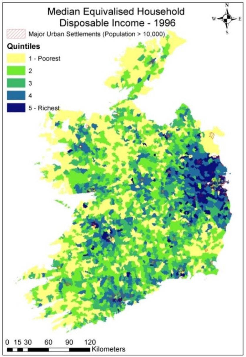
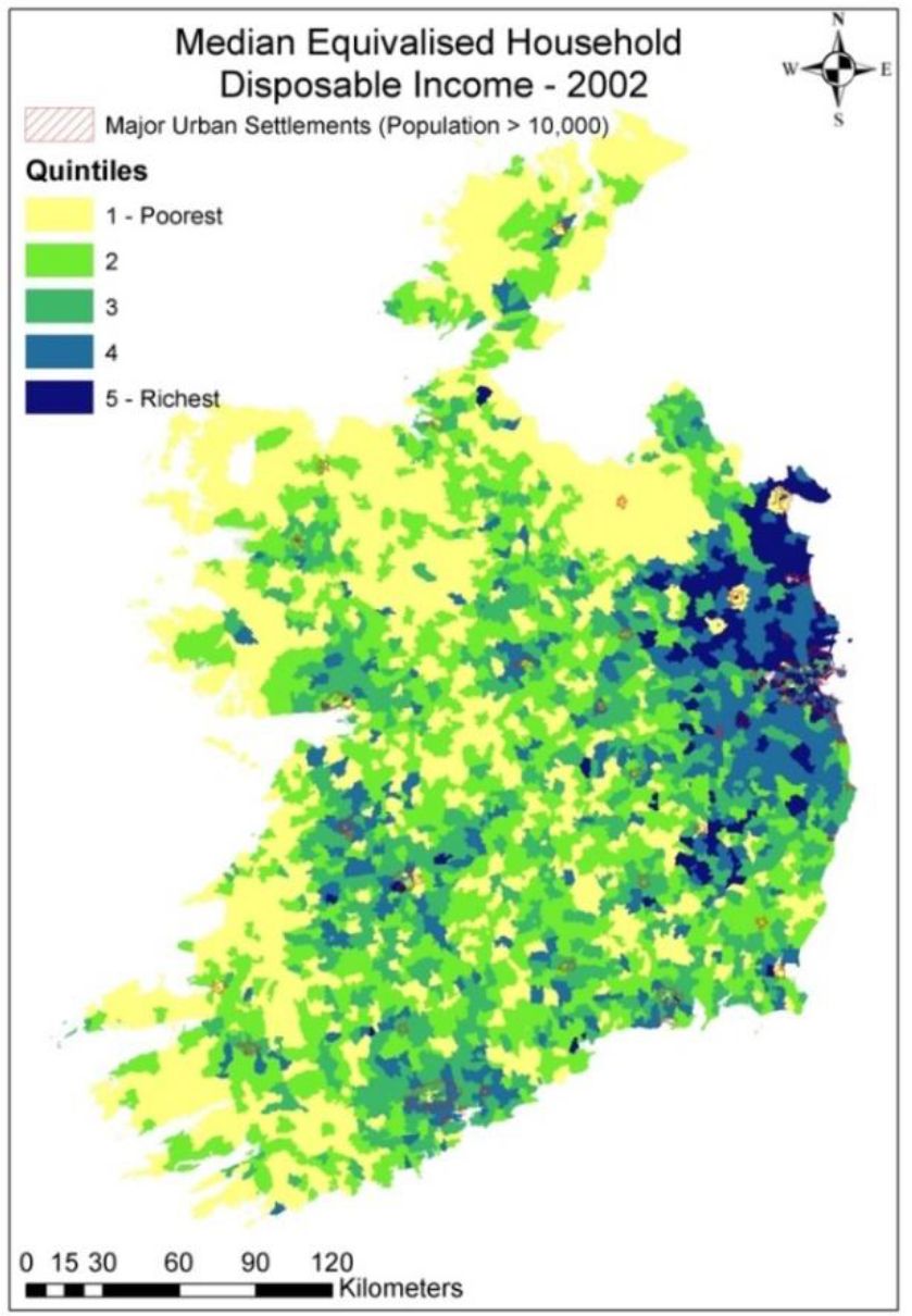
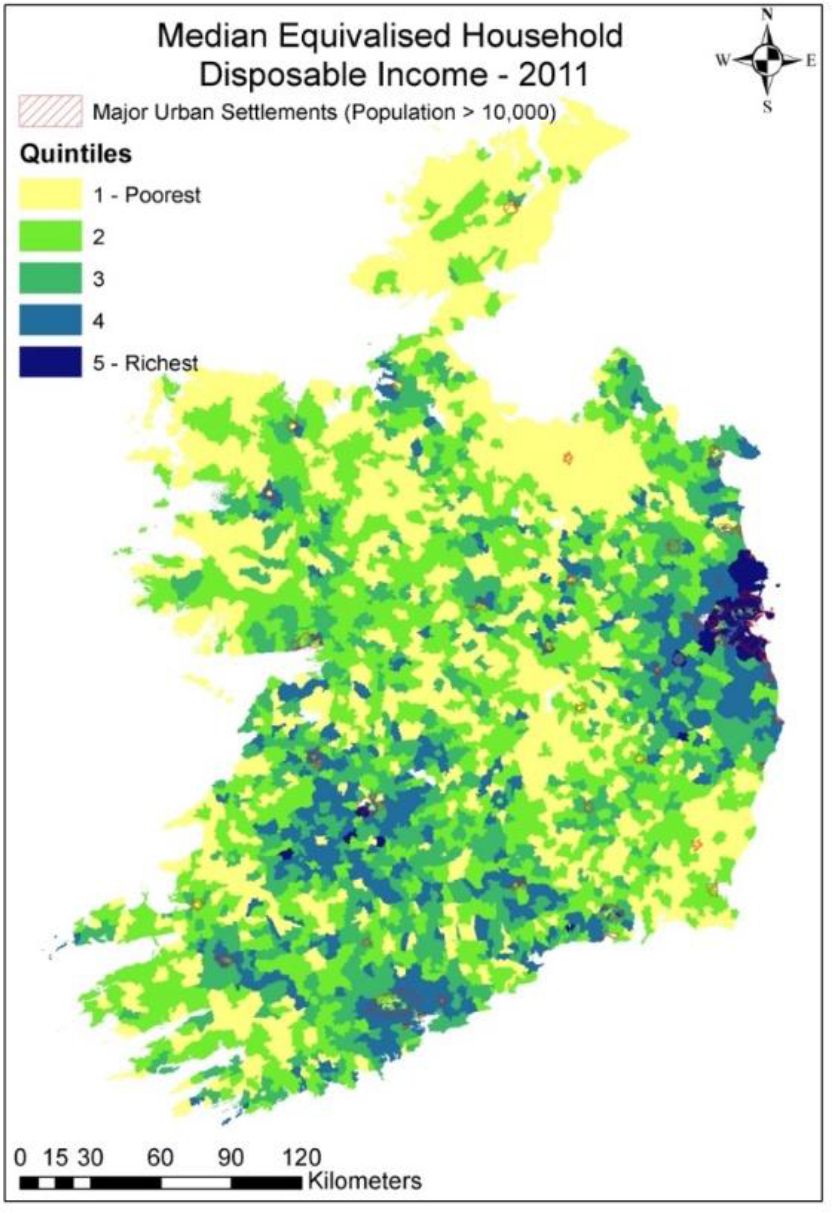
Our maps show the resulting spatial distribution maps of disposable income. Firstly, Figures 1 to 4 show the EDs divided into quintiles of median household equivalised disposable income.

Figure 1

Download asset Open asset

Figure 2

Download asset Open asset

Figure 3

Download asset Open asset

Figure 4

Download asset Open asset

There are some interesting results especially around the major urban settlements. If we look at the map for 1996 we can see that those in the commuter areas around Dublin are mostly in the top two quintiles. This covers quite a large area. The majority of areas with high levels of disposable income are centred on the major urban centres. This is what you would expect as these areas have better job opportunities, which in turn leads to higher salaries. There is a clear urban/rural divide. The EDs in the poorest quintile are for the most part a large distance from a major urban settlement, with the exception of county Louth.

As we move on to 2002 the GDA income landscape has changed. There is a clear shift towards the north of Dublin. High levels of income are also more concentrated around Dublin with even less EDs outside of the GDA in the top quintile. People seem to be willing to live in the suburbs and commuter counties around Dublin and commute into the city for employment. In 2006 the number of EDs outside of Dublin in the top quintile has reduced even further. Table 5 shows that population density in the top quintile is also increasing. This suggests Dublin City has become even more concentrated. It is attracting high levels of people in search of better opportunities. The south-west of the country has also seen an increase in the number in top quintile. While again the urban-rural divide is quite stark. Much of the centre and north of the map remains in the bottom quintiles. These areas are characterised by low population density, low levels of third level education and high unemployment. They also receive more in social benefits on average.

The final year 2011 has again seen a greater concentration in the GDA. A number of EDs in the commuter belt around Dublin have dropped out of the top quintile. We can also see that Cavan/Monaghan (North-Centre) is almost entirely in the bottom quintile. As mentioned earlier this area has the largest proportion of so called “ghost estates” and was particularly badly affected by the recession. Fortunes in the south-west of the country have continued to improve.

An examination of the breakdown of EDs in urban/rural as well as their quintile backs this up (Table 6). The more populated the settlement type the more likely an ED will belong to higher quintiles. Looking at those EDs in a rural area, 70% of all the population is in Q1 or Q2. The exception to the rule is Galway city where the majority are in Q3. A comparison between 1996 & 2011 shows that the gap between urban and rural has grown over time. There are now more people living in the urban areas in Q4 & Q5 and less people in Q4 & Q5 living in rural or small towns and villages.

Large changes in Irish society have taken place during this time period. Table 7 shows the breakdown of working population by industry of employment. We consider the top quintile (Q5) and the bottom quintile (Q1) as well as the movers. There has been a large move away from manual industries such as agriculture, construction and manufacturing towards more professional industry sectors like commerce, public administration and professional services (e.g. education). Most interestingly the difference is over time rather than between quintiles which is negligible.

The construction industry is particularly interesting as there was a large increase in employment in the industry followed by a sharp decline. In Forfas (2013) employment data in the construction sector was examined. In 2009 alone the number of unemployment construction workers increased by 190%, and construction workers accounted for 29% of all unemployment. Table 4 shows the number of new house completions⁴ broken down by census year. Put together with the employment figures in construction this goes towards explaining the reason behind the large numbers of construction workers unemployed in 2011. We can see this in Figure 5, as house completions begin to decrease in 2007, so too do employment figures in construction. There is however a lag of about 1 year before employment figures began to decrease rapidly.

Figure 5

Download asset Open asset

It is obvious from the maps that there is a continuing concentration of activity around the GDA. Even within the GDA itself the number of EDs in the commuter belt in the top quintiles has continued to decrease over time while at the same time the population density of the EDs in Dublin city in the top quintile has increased. From Table 5 we see that employment income in Dublin is considerably higher compared to the rest of the country. The increase in the level of opportunities in the area has proven attractive.

Table 5 shows the average values for Q1 & Q5 for the years 1996 and 2011. Population density in the top quintile has increased between the two years. There has been a convergence of people into the urban areas as they seek better opportunities. Levels of education have increased over time; even those in the bottom quintile have seen the percentage of adults with third level education increase. Employment is also higher in 2011, as is the share of people of working age. Unemployment however is also higher in 2011 as a result of the recession.

Youth deprivation has decreased while at the same time old age deprivation has increased. This would suggest an ageing population. The top quintile is made up of a high proportion of older people in 2011 compared to 1996 which would suggest that those over the age of 65 were less affected by the recession. Most of the analysis conducted is cross-sectional between areas. Table 8 shows the Thiel index I2 (Shorrocks, 1982). The Thiel index decomposes inequality into two components between and within variability. We can see that much of the variability is occurring within rather than between EDs. Although our maps show that there is a changing landscape across Ireland much of this change is occurring within EDs rather than between them. An examination of the tabulations of income by area shows that to be the case. Within an area we cannot say definitively whether an ED has more individuals in one particular quintile on the income distribution.

From our results we have seen an increase in concentration in and around Dublin City. This has largely been to the detriment of the rest of the country. Urban areas are vastly outperforming rural areas. The statistics of the areas in the bottom quintile which are largely rural are not promising. These areas are characterised by high levels of unemployment, low income and low levels of third level education. Equally there may be non-monetary reasons why individuals are choosing to live in these areas, such as better amenities and a better lifestyle/environment.

What our results have shown is that current policy is failing. Government has failed to control the concentration of economic activity around the GDA. The trends are worrying and have already led to a housing crisis particularly in the GDA. This crisis was inevitable given the increasing wages and property prices in these areas. Our Thiel index results show the high levels of inequality within rather than between EDs. Within an ED there are vast differences in income. Dublin has proven attractive to those with high levels of education who demand a higher wage. This has led to people converging on Dublin hence the increasing population density over time. Policy should look at addressing this issue by improving job opportunities in medium to small sized towns. This could be achieved by improving the infrastructure in these areas to bring them in line with the facilities etc. available in a major urban centre such as Dublin.

Policy can go some way towards improving the economic performance of a region. Removing the barriers around mobility of labour is one option (Marston, 1985, Armstrong and Taylor, 2000, Carlsen, 2000). Attractive living conditions; good services, high wages; have led to permanent differences in the wage and unemployment rate. It is difficult for income to increase in an area of high unemployment due to the excess in labour supply. The districts with the lowest incomes also tend to be the districts with the highest levels of unemployment. There is a spatial concentration of those most at risk of poverty. Increased investment in public housing in areas where there are better opportunities is one method of supporting the movement of people out of high poverty areas. Government subsidies can make it affordable for them to live in more prosperous regions and areas.

Centrifugal forces include high rents, commuting which then leads to congestion and supply of immobile factors (Fujita et al., 2001). Currently the Greater Dublin Area (GDA) is facing a crisis in this regard (increasing rents, congestion issues, and low property supply). The effect of these forces on disposable income warrants further investigation, for example, quantifying how much an average worker is spending each year on commuting costs and on renting a property.

using a spatial Microsimulation approach allows us to examine incomes at an individual and household level. This has enabled us to create an income distribution at a spatial level by firstly calculating the median equivalised household disposable income of an ED and then dividing this into quintiles taking into account the population of the EDs. Examining by urban/rural and over time we have observed the changing landscape in Ireland, a move of workers/people towards the major urban centres, the increase in wealth of these areas, the vast change in the breakdown of industry of employment and finally the change in the socio economic characteristics of the quintile groups.

This analysis includes an economically diverse period, represented by strong economic growth, a property bubble and subsequent collapse and recessionary period. Examining at the small area level has allowed us to track an area’s economic status over time and also the socio-economic and socio-demographic characteristics of its residents. our analysis shows the increasing regional imbalance between urban and rural areas. This gap has increased during the time period examined in this paper. Next steps involve examining ways in which this regional imbalance can be corrected.

1. 1
   Regional Economlcs & Policy

   1. H Armstrong
   2. J Taylor

   (2000)

   Regional Economlcs & Policy.

   • Google Scholar
2. 2
   Spatial microsimulation for rural policy analysis in Ireland: The implications of CAP reforms for the national spatial strategy

   1. D Ballas
   2. G Clarke
   3. E Wiemers

   (2006)

   Journal of Rural Studies 22:367–378.

   • Google Scholar
3. 3
   Immigrants in a booming economy: analysing their earnings and welfare dependence

   1. A Barrett
   2. Y McCarthy

   (2007)

   Labour 21:789–808.

   • Google Scholar
4. 4
   Going NUTS: The effect of EU Structural Funds on regional performance

   1. SO Becker
   2. PH Egger
   3. M Von Ehrlich

   (2010)

   Journal of Public Economics 94:578–590.

   • Google Scholar
5. 5
   New estimates of quality of life in urban areas

   1. GC Blomquist
   2. MC Berger
   3. JP Hoehn

   (1988)

   The American Economic Review pp. 89–107.

   • Google Scholar
6. 6
   Simulating Welfare and Income Tax Changes (SWITCH) The ESRI tax-benefit model

   1. T Callan
   2. C O’Donoghue
   3. C O’Neill

   (1996)

   Dublin: Economic Social Research Institute.

   • Google Scholar
7. 7
   Testing equilibrium models of regional disparities

   1. F Carlsen

   (2000)

   Scottish Journal of Political Economy 47:1–24.

   • Google Scholar
8. 8
   Accounting for cross-country income differences

   1. F Caselli

   (2005)

   Handbook of economic growth 1:679–741.

   • Google Scholar
9. 9
   Report of the Commission for the Economic Development of Rural Areas

   1. CEDRA

   (2013)

   CEDRA, Report of the Commission for the Economic Development of Rural Areas.

   • Google Scholar
10. 10
    SAPS Description of Contents

    1. CSO

    (2006)

    Central Statistics Office.

    • Google Scholar
11. 11
    http://www.cso.ie/en/media/csoie/releasespublications/documents/silc/2012/silc_2012.Pdf

    1. CSO

    (2014)

    Survey on Income and Living Conditions (SILC) 2012 [Online]. Accessed March 25, 2015.
12. 12
    Distribution of regional income and regional funds in Europe 1989–1999: an exploratory spatial data analysis

    1. S Dall’Erba

    (2005)

    The Annals of Regional Science 39:121–148.

    • Google Scholar
13. 13
    Shrink smarter? Planning for spatial selectivity in population growth in Ireland

    1. G Daly
    2. R Kitchin

    (2013)

    Administration 60:159–186.

    • Google Scholar
14. 14
    The fall of the Celtic Tiger: Ireland and the euro debt crisis

    1. D Donovan
    2. AE Murphy

    (2013)

    Oxford University Press.

    • Google Scholar
15. 15
    Microsimulation Methods and Models

    1. N Farrell
    2. K Morrissey
    3. C O’Donoghue

    (2012)

    Simulated Model for the Irish Local Economy, Microsimulation Methods and Models, London, Springer.

    • Google Scholar
16. 16
    Rural-urban migration, urban unemployment and underemployment, and job-search activity in LDCs

    1. GS Fields

    (1975)

    Journal of development economics 2:165–187.

    • Google Scholar
17. 17
    Ireland’s Construction Sector: Outlook and Strategic Plan To 2015

    (2013)

    Forfas, Ireland’s Construction Sector: Outlook and Strategic Plan To 2015, Dublin, Ireland.

    • Google Scholar
18. 18
    The spatial economy: Cities, regions, and international trade

    1. M Fujita
    2. PR Krugman
    3. A Venables

    (2001)

    The spatial economy: Cities, regions, and international trade, MIT press.

    • Google Scholar
19. 19
    Regional income inequality in selected large countries. IZA Discussion paper series

    1. A Heshmati

    (2004)

    Regional income inequality in selected large countries. IZA Discussion paper series.

    • Google Scholar
20. 20
    Catching up with the leaders: the Irish hare. Brookings papers on economic activity

    1. P Honohan
    2. B Walsh

    (2002)

    1–77, Catching up with the leaders: the Irish hare. Brookings papers on economic activity, 2002.

    • Google Scholar
21. 21
    Asset booms and structural fiscal positions: The case of Ireland. IMF Working Papers

    1. D Kanda

    (2010)

    1–23, Asset booms and structural fiscal positions: The case of Ireland. IMF Working Papers.

    • Google Scholar
22. 22
    https://openknowledge.worldbank.org/handle/10986/9144

    1. A Kilroy

    (2009)

    Intra-Urban Spatial Inequality: Cities as” Urban Regions” [Online]. Accessed August 15, 2013.
23. 23
    A haunted landscape: housing and ghost estates in post-Celtic Tiger Ireland. National Institute for Regional and Spatial Analysis (NIRSA) Working Paper

    1. R Kitchin
    2. J Gleeson
    3. K Keaveney
    4. C O’Callaghan

    (2010)

    59, A haunted landscape: housing and ghost estates in post-Celtic Tiger Ireland. National Institute for Regional and Spatial Analysis (NIRSA) Working Paper.

    • Google Scholar
24. 24
    The New Ruins of Ireland? Unfinished Estates in the Post-Celtic Tiger Era

    1. R Kitchin
    2. C O’Callaghan
    3. J Gleeson

    (2014)

    International Journal of Urban and Regional Research 38:1069–1080.

    • Google Scholar
25. 25
    Principles of economics: an introductory volume

    1. A Marshall

    (1920)

    Principles of economics: an introductory volume.

    • Google Scholar
26. 26
    Two views of the geographic distribution of unemployment

    1. ST Marston

    (1985)

    The Quarterly Journal of Economics pp. 57–79.

    • Google Scholar
27. 27
    Spatial Justice and the Irish Crisis

    1. D Meredith
    2. JP Faulkner

    (2014)

    The nature of uneven economic development in Ireland, 1991–2011, Spatial Justice and the Irish Crisis, Dublin, Ireland, Royal Irish Academy.

    • Google Scholar
28. 28
    Revisiting the National Spatial Strategy ten years on

    1. D Meredith
    2. C Egeraat

    (2013)

    Administration 60:3–9.

    • Google Scholar
29. 29
    Examining access to GP services in rural Ireland using microsimulation analysis

    1. K Morrissey
    2. G Clarke
    3. D Ballas
    4. S Hynes
    5. C O’Donoghue

    (2008)

    Area 40:354–364.

    • Google Scholar
30. 30
    Spatial microsimulation for rural policy analysis

    1. K Morrissey
    2. C O’Donoghue

    (2013)

    Validation Issues and the Spatial Pattern of Household Income, Spatial microsimulation for rural policy analysis, Springer.

    • Google Scholar
31. 31
    Using Simulated Data to Examine the Determinants of Acute Hospital Demand at the Small Area Level

    1. K Morrissey
    2. C O’Donoghue
    3. G Clarke
    4. J Li

    (2013)

    Geographical Analysis 45:49–76.

    • Google Scholar
32. 32
    National spatial strategy for Ireland 2002-2020: people, places and potential

    1. NSS

    (2002)

    Department of the Environment and Local Government Ireland.

    • Google Scholar
33. 33
    Spatial microsimulation for rural policy analysis

    1. C O’Donoghue
    2. D Ballas
    3. G Clarke
    4. S Hynes
    5. K Morrissey

    (2013)

    Spatial microsimulation for rural policy analysis, Springer.

    • Google Scholar
34. 34
    Regional income estimates for Ireland, 1995

    1. E O’Leary

    (1999)

    Regional Studies 33:805–814.

    • Google Scholar
35. 35
    The Microsimulation Unit. MU/RN/26

    1. C O’Donoghue

    (1998)

    University of Cambridge: Department of Applied Economics.

    • Google Scholar
36. 36
    http://www.oecd.org/eco/growth/OECD-Note-EquivalenceScales.pdf

    1. OECD

    (2014)

    OECD: Note on Equivalence Scales [Online]. Accessed March 25, 2015.
37. 37
    Wages, rents, and the quality of life

    1. J Roback

    (1982)

    The journal of political economy pp. 1257–1278.

    • Google Scholar
38. 38
    The determinants of agglomeration

    1. SS Rosenthal
    2. WC Strange

    (2001)

    Journal of Urban Economics 50:191–229.

    • Google Scholar
39. 39
    Evidence on the nature and sources of agglomeration economies

    1. SS Rosenthal
    2. WC Strange

    (2004)

    Handbook of regional and urban economics 4:2119–2171.

    • Google Scholar
40. 40
    Bridging the economic divide within countries: A scorecard on the performance of regional policies in reducing regional income disparities

    1. R Shankar
    2. A Shah

    (2003)

    World Development 31:1421–1441.

    • Google Scholar
41. 41
    Inequality decomposition by factor components

    1. AF Shorrocks

    (1982)

    Econometrica: Journal of the Econometric Society pp. 193–211.

    • Google Scholar
42. 42
    Consumption and social welfare: Living standards and their distribution in the united States

    1. DT Slesnick

    (2001)

    Cambridge university Press.

    • Google Scholar
43. 43
    Regional Income Inequality

    1. E Sommeiller

    (2006)

    University of Delaware.

    • Google Scholar
44. 44
    An urban–rural classification for health services research in Ireland

    1. C Teljeur
    2. A Kelly

    (2008)

    Irish Geography 41:295–311.

    • Google Scholar
45. 45
    Living in Ireland Survey – Technical Overview

    1. D Watson

    (2004)

    UCD.

    • Google Scholar
46. 46
    Ireland’s economic crisis: The good, the bad and the ugly. Working Paper Series

    1. K Whelan

    (2013)

    UCD Centre for Economic Research.

    • Google Scholar

Author details

1. Paul Kilgarriff

   National Centre for Geocomputation, Maynooth University, Ireland

   For correspondence

   p.kilgarriff1@gmail.com

2. Cathal O’Donoghue

   Teagasc Rural Economy and Development Programme, Mellows Campus, Ireland

   For correspondence

   cathal.odonoghue@teagasc.ie

3. Martin Charlton

   National Centre for Geocomputation, Maynooth University, Ireland

   For correspondence

   martin.charlton@,nuim.ie

4. Ronan Foley

   Institute Department of Geography, Maynooth University, Ireland

   For correspondence

   ronan.foley@nuim.ie