Constructing a synthetic city for estimating spatially disaggregated heat demand
- Technical Urban Infrastructure Systems Group, HafenCity University, Germany
- Article
- Figures and data
-
Jump to
- Abstract
- 1. Introduction: Creating a synthetic building stock
- 2. Data: Census (2011) & micro census (2010)
- 3. Heating demand
- 4. Simulation: Using gregwt to reweight the microcensus
- 5. Benchmarking to different aggregation units
- 6. Results: Heating demand
- 7. Next steps: Integrated reweighting
- 8. Conclusions: Creating rich data-sets for the Urban simulation community
- Footnotes
- Annex
- References
- Article and author information
Abstract
We present a procedure for creating a spatially referenced building stock with population living therein “a synthetic city” for the case of Germany. The level of spatial disaggregation is the European NUTS–3 level for which data from the newest census (2011) exist. Our application is on the estimation of heat demand.
We use the German microcensus (2010) which contains both: (a) detailed sociodemographic characteristics of individuals and (b) detailed information on the type of buildings in which these individuals live. With this data we can generate not only a synthetic population but also a synthetic building stock. The microcensus records the construction year and number of dwelling units of buildings. This allow us to classify the buildings for the estimation of heat demand.
This procedure has two major advantages: (1) there exist many models for the estimation of heat demand at building level, we can make use of these models, and (2) with the microcensus as the only required data source we are able to estimate heat demand at a spatially disaggregated level for the entire country.
We conclude our paper with an internal validation of the microsimulation model by means of the Total Absolute Error TAE and present the first results from this model aggregated at the NUTS–3 level for the entire country. We briefly discuss the observed patters of the results and attempt to hypothesize on the reasons behind this patterns. We also discuss the difficulties of an external validation of this model and how we can address them in the future.
1. Introduction: Creating a synthetic building stock
The development of a synthetic city representing the urban fabric of urban agglomerations has proved helpful for the development of urban models, the focus of this endeavour has been the use of remote sensing data or other type of image and laser data available at a low aggregation level in order to generate urban structures. Laycock and Day (2003) presents an overview of used data sources and methods for the generation of urban structures. Parish and Müller (2001) used a procedural approach based on L-systems to generate urban structures. The authors use different maps as input for the generation of the geometrical representation of the city. Our aim is to expand these methods by creating appropriate data regarding the building stock and the population living and working on this building stock that can be used as input to these models for the generation of synthetic cities. Kang, Ma, Tong, and Liu (2012) create a set of synthetic cities in order to asses the relationship between urban morphologies and human mobility. Kii, Akimoto, and Doi (2014) develop a simple synthetic city for the assessment of urban transport policies, the authors generate the synthetic city and use this data as input for a land use model, subsequently the authors apply the postulated policies to the model in order to asses them. The authors argue in favor of including user behaviour in urban models. Farber, Neutens, Miller, and Li (2013) generate eighty different synthetic cities in order to analyze the Social Interaction Potential of these environments based on commuting patterns and land use distribution. Bagchi, Sprintson, and Singh (2013) use a synthetic city for the simulation of fire dispersion on an electrical distribution grid, in this case the authors represent the building stock and an electrical grid. Mei et al. (2015) develop a synthetic city in order to study the diffusion of infectious diseases. The authors use the synthetic city in order to understand the outbreak of influenza in dense populated urban areas in China. In this case the authors do not require a detailed description of the building stock geometry but only the building use. Stötzer, Hauer, Richter, and Styczynski (2015) define a simple synthetic city for the estimation of the potential load shift of commercial and residential electricity demand. Because the authors are only interested in electric consumption, they do not create a geometrical representation of the building stock nor do they have any type of geo-reference in the synthetic city. In this paper the authors define the electric consumption as a function of household size. Many of the examples presented above could be implemented on a more realistic environment describing the characteristics of the building stock and the population living on them.
The development of a robust method for the creation of synthetic cities representing specific urban agglomerations with known population aggregates constitutes the scope of this paper. This paper presents first results from this endeavour. It is shown the developed method for the representation of a synthetic city, describing individuals and the characteristics of their households and the building they reside on. Here we do not discuss in detail the pursued method for the representation of geo-referenced geometrical objects. We present some discussion regarding the different alternatives to generate a geometrical representation of the synthetic city extending the methods described in this paper.
The method used in this analysis is a spatial microsimulation method. Microsimulation, introduced by Orcutt et al. (1977) is a commonly used method among social scientist used to simulate a large range of social phenomena at a micro-level. The first step of this method is normally the generation of a synthetic population representing the population under analysis. The spatial microsimulation methodology extends this concept by allocating estimated synthetic populations to geographical areas (Clarke & Holm, 1987). This simulation method is applied by a large number of disciplines. Brown and Harding (2002) and Smith, Pearce, and Harland (2011) argue the use of this type of models for the analysis of health systems, the modeling of resources consumption is addressed by Williamson, Clarke, and McDonald (1996); Williamson, Mitchell, and McDonald (2002) for the estimation of water consumption and Chingcuanco and Miller (2012) and Muñoz H. and Peters (2014) for the estimation of energy demand. Many transport models use this approach for the generation of synthetic populations (Farooq, Bierlaire, Hurtubia, & Flötteröd, 2013). For overview of spatial microsimulation models, its applications and methods see (Tanton, 2014; O’Donoghue, Morrissey, & Lennon, 2014). In this paper we make use of an “generalised regression weighting” (GREGWT) algorithm to create a synthetic population. We use the available R library (Muñoz H., Vidyattama, & Tanton, 2015a), implementing the GREGWT algorithm, originally developed by the Australian Bureau of Statistics (ABS) (Bell, 2000). This algorithm is used by the National Center for Social and Economic Modeling (NATSEM) on their spatial microsimulation model spatialMSM (Tanton, 2007).
The presented paper is structured as follows: Section 2 presents and describes the used data for the analysis and the undertaken steps in preparing the data for the simulation, the next section, Section 3, describes the computation method to estimate heat demand for each individual on the microcensus and the assumptions made for this computation. Section 4 describes the method used for the reweighting of the microcensus with the computed heating demand values. We benchmark the survey to benchmarks describing individuals, dwelling units and buildings. These process is described under Section 5. The results from the simulation are described and discussed under Section 6. On Section 7 we highlight the benefits and shortcomings of the developed method and propose extensions to this method in order to address some shortcomings of the applied method. In the last section, Section 8, we make a brief resume of the paper, its main findings and possible applications for the infrastructure planning of urban environments.
2. Data: Census (2011) & micro census (2010)
In the literature we find two type of models for the construction of synthetic data: (1) synthetic reconstruction and (2) reweighting (Rahman, 2008). The GREGWT algorithm forms part of the latter group. This algorithm is a deterministic method that reweights a sample survey to match aggregated statistics available at small geographical areas.
In order to create a synthetic population with the GREGWT method we need two data sets: (1) a survey sample containing individual records and (2) aggregated statistics available at a NUTS–3 geographical level. For the purpose of this simulation we want to create a synthetic population describing the demographic characteristics of the individuals as well as characteristics of the dwelling units these individuals reside on. In order to generate such a data set we select data describing three different aggregation units: (1) individuals, (2) household/dwelling units and (3) buildings. Table 1 list the used variables from the two data sets.
Used benchmarks from the 2011 Census and corresponding micro census attributes.
| MC Code* | Census Code | Unit** | Description |
|---|---|---|---|
| EF1 | / | / | Federal State (NUTS 2) |
| EF952 | / | Person | Weight |
| EF44 | ALTER_KURZ | Person | Age (five classes of years) |
| EF49 | FAMSTND_AUSF | Person | Marital status (in detail) |
| EF46 | GESCHLECHT | Person | Sex |
| EF20 | HHGROESS_KLASS | Person | Size of private household |
| EF368 | STAATSANGE_KURZ | Person | Citizenship |
| EF492 | WOHNFLAECHE_20S | Dwelling | Floor area of the dwelling (20m2 intervals) |
| EF494 | BAUJAHR_MZ | Building | Year of construction (microcensus classes) |
| EF635 | ZAHLWOHNGN_HHG | Building | Number of dwellings in a building |
-
*
Micro Census Code
-
**
Refers only to Census
The synthetic population is represented as the reweighted German micro census, we reweight this survey with help of an R library implementing the GREGWT method (Muñoz H., Vidyattama, & Tanton, 2015a). The GREGWT method is classified as a deterministic reweight method (Tanton, Williamson, & Harding, 2014). Deterministic reweighting methods aim to reweight a survey to match known aggregated values of geographical areas. The sample size and availability of the data of these geographical areas vary between countries. For the European Union a standard incorporating the different national definitions exist. This is the Nomenclature of Territorial Units for Statistics (NUTS1) standard. This nomenclature describes four hierarchies: (0) national territories; (1) NUTS–1; (2) NUTS–2; and NUTS–3. A reweighting of a national survey could be implemented at any of the NUTS levels. Depending on the research question a suitable geographical area should be selected. These geographical areas have different names on each country and the authors referee them according to the use case location. These areas are known as: (a) Summary Files in the U.S.; (b) Profile Tables or Basic Summary Tabulations (BSTs) in Canada; (c) and Small Area Statistics in the U.K. (Pritchard & Miller, 2012).
3. Heating demand
The heating demand is computed for each individual in the microcensus. For the computation of heating demand of each individual we need to consider the characteristics of the building stock. In order to take these characteristics into account we make use of the IWU building typology (Diefenbach, Cischinsky, Rodenfels, & Clausnitzer, 2010; Loga, Diefenbach, & Born, 2011). We classify each individual to one of the 36 IWU building typology types. For the estimation of heating demand per dwelling unit we need to take into account the household size and divide the estimated heating demand by its household size. For a household with four members we compute the heating demand for each member of the family as kWh per dwelling unit m2. In order to get the heating demand of the dwelling unit we sum the heating demand of each member divided by household size. On this model the computed heating demand of each family member is the same, nonetheless if we where to take user behaviour into account this values would differ from each other (Muñoz H., 2014). This is necessary because the computed heating demand is the estimated heating demand per squared meter of dwelling unit. An alternative to this would be to divide the dwelling unit area by household size.
In order to classify the microcensus into the building types we use three parameters from the microcensus: (1) building construction year, (2) dwelling unit size, and (3) number of dwelling units per building. A summary of the rules applied to the microcensus to achieve this classification are listed in Table 4.
The main parameter used for the classification is the building construction year. We use the number of dwelling units to differentiate between single family houses and multi-family houses. Finally, the dwelling unit size multiplied by the number of dwelling units is used to distinguish between small mutli-family housed, large multifamily houses and high rise buildings. The specific heating values of the IWU building typology used in this analysis are listed in Table 2.
IWU-de building typology matrix for Germany.
| <1859 | 1860–1918 | 1919–1948 | 1949–1957 | 1958–1968 | 1969–1978 | 1979–1983 | 1984–1994 | 1995–2001 | 2002–2009 | |
|---|---|---|---|---|---|---|---|---|---|---|
| EFHa | 183 | 180 | 164 | 181 | 146 | 155 | 118 | 132 | 110 | 88 |
| RH | 153 | 137 | 156 | 106 | 127 | 127 | 98 | 78 | 86 | |
| KMH | 190 | 143 | 168 | 156 | 129 | 134 | 118 | 122 | 92 | 79 |
| GMH | 127 | 144 | 142 | 131 | 117 | |||||
| HH | 114 | 113 |
-
source: (Loga et al., 2011) (a) Speci..c Heat demand (spez. Wärmebedarfskennzahl) [kWh/m2a] (EFH) Single family house “Einfamilienhaus”; (RH) Terrace house “Reihenhaus”; (KMH) Apartment house “Mehrfamilienhaus”; (GMH) Large apartment house “Großes Mehrfamilienhaus”; (HH) High-rise “Hochhaus”;
The advantage of using a building typology for the estimation of heating demand is that we don’t need to take assumptions about the building geometry. This is because the values listed under the building typology represent specific heating demand. In order to compute the absolute heating demand we simply multiply this value by the building square meters. In order to explicitly account for building geometry we need to allocate individuals to a digital cadastre describing the building properties, see (Muñoz H. & Peters, 2014).
The disadvantages of using the digital cadastre for the computation of heating demand are: (1) the digital cadastre of other type of building information data are not as homogeneous as demographic data and building typologies, there are many building typologies available for Europe (Caputo, Costa, & Ferrari, 2013; Hrabovszky-Horváth, Pálvölgyi, Csoknyai, & Talamon, 2013; Kragh & Wittchen, 2013; M. K. Singh, Mahapatra, & Teller, 2013; Dall’O’, Galante, & Torri, 2012; Dascalaki, Droutsa, Balaras, & Kontoyiannidis, 2011; Balaras et al., 2007), as for its demographic data. (2) the complexity of data representing the building stock makes it difficult to make projections into the future, Muñoz H., Vidyattama, and Tanton (2015b) present an application of a synthetic building stock projected into the future with a simplified building geometry.
4. Simulation: Using gregwt to reweight the microcensus
The aim of the GREGWT is to reweight a survey implementing method number 5 from A. Singh and Mohl (1996). Tanton, Vidyattama, Nepal, and McNamara (2011) makes a detailed description of the algorithm and its applications. Rahman, Harding, Tanton, and Liu (2013) presents an application of the GREGWT algorithm for the construction of synthetic population, the authors show a good performance of the method for the estimation of household stress in Australia. The mathematical description of the GREGWT algorithm presented below is taken from Rahman, Harding, Tanton, and Shuangzhe (2010) and the algorithm description from Muñoz H., Tanton, and Vidattama (2015).
Aim of the GREGWT algorithm is to find a set of new weights w that can be used to match a survey X to a set of given benchmarks T so that (e.g. small area aggregates) by minimizing the weight difference between these new weights w and the sample design weights d from the survey. For the distance D between design and estimated weights the GREGWT algorithm makes use of the truncated Chi-Squared distance function, represented in Equation 1.
The equation needed to minimize the weight distance constraint to some given marginal totals of a geographical area (T) can be expressed as the Lagrangian function of the Chi-Squared function, as follows:
By differentiating (1) with respect to wj and applying the first order condition, we have:
With this equation we can formulate an equation for the new weights. Where .
The new weights computed by the GREGWT algorithm are float values. Without any restrictions the algorithm will produce negative weights, both implementations of the algorithm introduce boundary constrains as user input. The user can define an upper and lower bound, if the algorithm computes weights outside these bounds the weights will be truncated to the corresponding bounds. In this case the algorithm will iterate with the new computed weights until a predefined convergence parameter is met or until there is no improvement in the iteration.
The implementation of the GREGWT algorithm in the R language adds an extra calibration method for the new estimated weights. This last process makes sure that the sum of the new weights is equal to the total population of the specific area. Equation 5 shows the alignment used to calibrate the resulting weights.
Where wo are the new calibrated weights, p is the population total and w are the computed new weights from the GREGWT algorithm.
5. Benchmarking to different aggregation units
The defined benchmarks for the reweighting of the survey are aggregated by different units: (1) Individuals, (2) Families, and (3) Buildings (see Table 1 and Section 2). The used R implementation of GREGWT algorithm is able to perform an integrated reweight. This is important for maintaining unit aggregations, f.ex. to maintain the family structure given by the survey. Nonetheless, this does not allow us to benchmark to different aggregation units. Attempts to address this issue exist in the literature, Guo and Bhat (2007) benchmark an initial survey to household characteristics and fit the result to individual benchmarks in the integerization2 of the weights via a Monte Carlo process. This method allows to “benchmark” to both aggregation units. The disadvantage of this approach relies on its inegerization process, this process is only required for the construction of agents at the cost of a decline of the algorithm performance. For the presented simulation we do not require individual agents and therefore any form of integerization would be contra productive for the final result. For a description of other similar approaches see Pritchard and Miller (2012) and Ma and Srinivasan (2015). Pritchard and Miller (2012) propose a “Conditional Monte Carlo Synthesis Procedure” to fit the synthetic population to both: household and individual benchmarks. Again this procedure assumes an integerization of the survey. As described above we aim to develop a method that does not require an integerization step in order to avoid: (a) a decline in the performance of the algorithm, (b) an explosion of computational time, and (c) introduction of a stochastic element to a deterministic approach. Ma and Srinivasan (2015) developed another method to create a synthetic population: “fitness-based synthesis” (FBS). The method presented by Ma and Srinivasan proposed the computation of two fitness values expressing the adding and subtracting probability of individuals from the random selected population from the reweighted population survey.
The GREGWT algorithm needs to transform the input matrix X (micro census) to a binary matrix, each 1 on the matrix corresponds to an individual. This works well if we benchmark the survey to aggregates counting individuals (e.g. number of individuals on age category 18 to 20) but fails if we try to benchmark to an aggregate counting dwelling units (e.g. number of dwelling units with floor space of 60 m2). We need to control for this difference. With the available information of the input survey we can manipulate the binary matrix in order to make the benchmarking to different aggregation units possible. For variables benchmarked to dwelling units we divide them by household size, an individual with household size 3 will get a 1/3 instead of 1 in the X input matrix. For all variables counting buildings we divide the values by the household size and number of dwelling units, the same individual living in a building with 6 dwelling units will have a value of 1/3/6. This calibration is formalized in Equation 6 and 7, where HH is household size and DU is number of dwelling units.
With this simple modification of the survey we are able to benchmark the input survey to three aggregation levels. In theory this method allows us to benchmark to any number of aggregation units.
6. Results: Heating demand
In this section we present the main results from the performed spatial microsimulation. The results show the estimated heating demand for the German residential sector. First we present an internal validation of the spatial microsimulation model and the resulting heating demand. The results are aggregated back to the geographical areas in order to visualize them.
In order to internally validate the model we compare the results at the NUTS–3 level. We compare the output results with the benchmarks used in the reweighting process. For the comparison we make use of the Total Absolute Error (TAE) and the Percentage Absolute Error (PTAE), two measures of the model internal error. The TAE is the absolute difference between the simulated and observed T benchmarks, the PTAE is an extension of the TAE measure. The PTAE divides the computed TAE by the total population pop of the geographical area i. The mathematical expressions of both measures are expressed below.
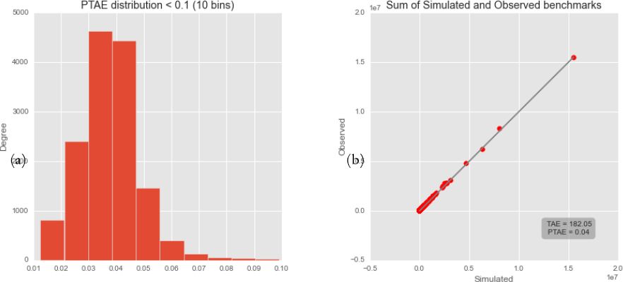
The resulting PTAE values show a very low miss-allocation of individuals at this aggregation level. There are only four areas with a PTAE value higher than 0.2% and 52 areas with a value higher than 0.1%. Figure 1 shows: (a) the distribution of the PTAE values for all simulation areas; and (b) a scatter plot comparing the observed and simulated marginal sums. Figure 1b compares the simulated and observed small area benchmarks. The plot shows a very good performance of the estimation. The mean TAE of the estimation of 182.05, this means that on average 182.05 individuals are misrepresented on a small area. In order to compared the misrepresentation of individuals per small are we divide this value by the total population on the corresponding area PTAE. The mean PTAE value is of 0.04. This means that on average 0.04% of individuals are misrepresented on the small areas.

(a) Distribution of PTAE and (b) difference between estimated and simulated population.
The Internal validation of the model shows extremely good results, these results do not reflect on the accuracy of the estimated heating demand. An external validation of the model is necessary in order to validate the estimation of heating demand. This paper shows that the use of a spatial microsimulation model for the estimation of heating demand at low aggregation levels is possible. The underlying model used for the estimation of heating demand has not yet been validated, still the estimation is able to show plausible differences in heating demand between small geographical areas. This method can be applied at a city level, differentiating the heating demand at a neighbourhood level.
An external validation of the model is not possible because energy consumption data is not available at this disaggregation level. Available energy consumption data exist at a higher aggregation level. This data does not differentiate between consumption sectors, neither does it between primary and end-energy consumption. Our model simulates residential end-heating demand. There is also a difference between heating demand and heating consumption, our model does not consider efficiency rates of heating supply infrastructure. Further steps are planned to make an external validation possible. The first step we envision towards a validation of estimated heating demand is the integration of the non residential sector to the model. With an estimate of the non residential sector we might be able to validate the sum of residential and non residential heating demand at a higher aggregation level. We also plan to include efficiency rates of the underlying heating supply infrastructure as well as the energy carrier used to supply the heating.
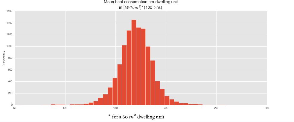
In order to show the results in a more meaningful way we divide the estimated total heating demand by the number of dwelling units in each geographical area and by a constant (60) representing the average dwelling unit size in m2 for Germany3. The resulting specific heating demand allows us to asses the performance of the model. The distribution of this value for all simulation areas is plotted on Figure 2, the values and distribution shown in this plot are consistent to known consumption values for the German building stock.

Mean heating consumption per dwelling unit.
We present two figures showing the estimated heating demand at a NUTS-3 level. The first map (Figure 3) shows the distribution of specific heating demand for the entire country. The second map shows the detail of four specific areas of Germany. In addition to the estimated heating demand we plot urban agglomerations retrieved from Landsat images, we make use of the GADM dataset containing this information (Hijmans et al., 2014).
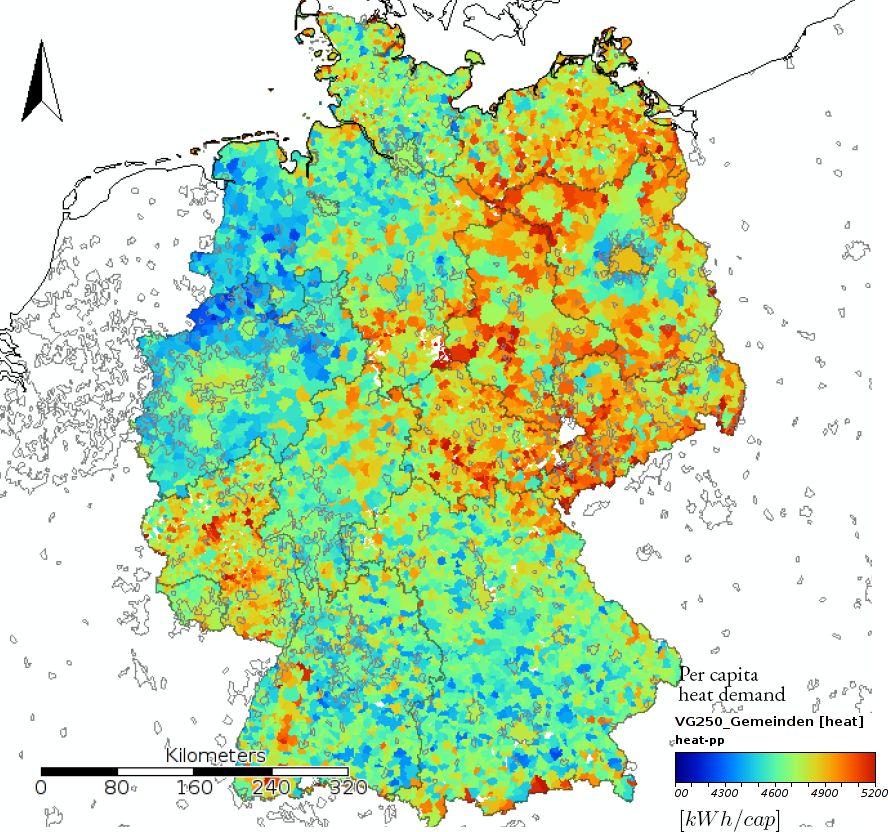
Simulated heat demand for Germany at a NUTS-3 level as per capita heat demand in kWh/cap.
On the first map (see Figure 3) we can identify a differentiation between West- and East-Germany. The specific heating consumption is higher in East-Germany. The specific heating consumption on East-Germany is higher because the building stock on this part of Germany is older and less energy efficient. This regional differentiation on heating demand shows that the presented model is sensitive to regional characteristics of the building stock. There is a big difference between East and West regarding the heating supply infrastructure. The share of households connected to a district heating network in East-Germany is much higher than in West-Germany.
Also the construction quality of the building stock differs significantly between these regions. This clear differentiation between small areas shows that the model is able to correctly capture the differences of the building stock.
The second map (Figure 4), showing a detail of the distribution of heating demand for the two largest cities in Germany: (a) Berlin and its surroundings, (b) Hamburg and its surroundings and two urban agglomerations: (c) the south-east part of North Rhine-Westphalia “Nordrhein Westfalen” and (d) Thuringia “Thüringen”, a federal state of East-Germany. In the case of the German cities, Berlin and Hamburg, the official NUTS–3 level is equivalent to the NUTS–2 and NUTS–1 level. Both areas have a disproportional large population size compared to all the other geographical areas. Statistics at a lower aggregation level are available for both cities and a second reweighting algorithm could be perform for these two areas separately. In both cases we see that the areas corresponding to the cities have a higher specific heating demand and the peripheries show a lower specific heating demand, we find an explanation for this differentiation in the construction year of the corresponding building stock. We expect to have an old building stock within the historical urban fabric of the cities, this part of the city will be well within the corresponding geographical area. Both cities have outgrown the boundaries of these geographical areas. The development of urban settlements at the periphery of the city, constructed in more recent years, are constrained to newer building codes regulating the heating transmission losses of the building shell and therefore consuming less heat.
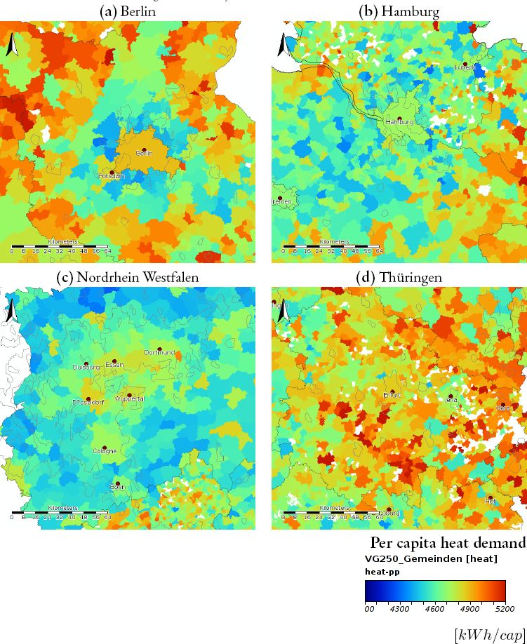

Simulated heat demand for selected regions of Germany.
We see a similar effect on the large urban agglomeration of North Rhine-Westphalia (see Figure 4c), the high values of heating demand correspond to the original settlements in the region. These settlements have the oldest building stock in the region. Large part of these settlements are under heritage protection, making the retrofit of the buildings extremely expensive and difficult. We can’t see this differentiation on the East-German urban agglomeration in the Thuringia state (see Figure 3d). The urban agglomeration is not as big as in North Rhine-Westphalia and the urban and population growth hasn’t been as big as in other German regions. In the case of North Rhine-Westphalia we see the opposite phenomena in which more rural areas in the periphery have higher consumption values.
The results presented in this paper show that an estimation of heating demand at this level of aggregation with relative little input data is possible. Future developments of the models aim to integrate projections of the heating demand consumption at the same area of aggregation. A theoretical background to perform a projection of heating demand with a spatial microsimulation model exists (Muñoz H., Vidyattama, & Tanton, 2015b). Muñoz H., Vidyattama, and Tanton (2015b) project the heating demand at a low aggregation level for the city of Hamburg using a spatial microsimulation model. Recent developments show an alternative method to project heating demand by simulating retrofits through the manipulation of the input weights of the micro census (Muñoz H., Tanton, & Vidattama, 2015). This method presents a clear advantage while simulating and projecting heating demand for the entire country at a low level of aggregation because we do not have to make assumptions for the projection of retrofit levels at a low level of aggregation. A possible implementation of this method is to align the initial weight distribution to proposed policies implemented at a federal level. In this scenario the aggregated retrofit rates are defined at a federal level and the allocation of these retrofits could be simulated as function of demographic characteristics at a lower geographical level.
7. Next steps: Integrated reweighting
The next envisioned step is to group the synthetic individuals into: (a) households and (b) into buildings. The advantage of grouping individuals into single buildings are: (1) the ability to represent energy consumption at a building level and (2) the possibility to geo-reference these buildings at a finer spatial resolution.
One of the applications for this synthetic data is the dimensioning and planning of decentralized energy supply systems. In order to make data usable for this application we need to represent energy demand at a finer spatial resolution. We may achieve this by obtaining aggregated benchmarks at a finer spatial resolution, this may not be possible due to data protection concerns. For this reason we want to develop new methods to further disaggregate heating consumption values. For this disaggregation we see two possible paths, the first step for both paths is the grouping of individual data into buildings.
The first approach makes use of the digital cadastre. The problem of this method is that a digital cadastre may not always be able for the desire area, this is specially true for rural areas. The second approach makes use of satellite images for the computation of spatial probability distributions of relevant building parameters (e.g. density, construction year, etc.) and stochastically allocated buildings to build up areas based on the computed spatial probabilities. The advantage of this method is that satellite images are available for the entire world, making the transferability of the method higher.
With a more efficient building stock in place the roll of user-behaviour will take a dominant place in the estimation of heating demand (Hong, D’Oca, Turner, & Taylor-Lange, 2015). The presented method already solves a common problem of urban models aimed at the estimation of residential heating demand with an explicit consideration of human behaviour, this is the allocation of families to the building stock. Muñoz H. and Peters (2014) use a spatial microsimulation model to describe households and the building characteristics they reside on for the estimation of heating demand varying user related parameters on the model according to the demographics of the user. A more elaborated approach is presented by Muñoz H. (2014), in this paper the author enriches the German micro census with a time-use survey for the generation of household schedules, these schedules are used as input in a thermal simulation model.
8. Conclusions: Creating rich data-sets for the Urban simulation community
The presented method describes a process to represent core characteristics of the building stock in an abstract fashion without fully describing, neither the real building geometry not an accurate location of the individual buildings. We make use of a new R library (Muñoz H., Vidyattama, & Tanton, 2015a) for the reweighting of the German micro census survey (2010) to small geographical areas, corresponding to the European NUTS-3 level. Available aggregated data regarding demographic information as well as information on the building stock are available at this level from the last German census (2011). In order estimate heat demand at a micro level we classify each individual in the micro census to a building type. We make use of a well established building typology for this classification (Loga et al., 2011). Because we know the dwelling unit size of every individual in the micro census we are able to transform the specific heat demand provided by the building typology into an absolute value, we control this value by household size, dividing the absolute estimate heat demand by the household size of each individual.
We make use of an innovative feature of the R library which allows us to benchmark the micro census to three different levels of aggregation: (1) individuals, (2) households and (3) building units. Preliminary results from the simulation are presented as maps at the NUTS-3 level. On these results we are able to identify a distinction between East and West Germany as well as a distinction between historical urban agglomerations, with a high heat demand, and new developments in the suburbs, with a more moderate heat demand. We conclude this paper by offering the reader a prospective on the challenges ahead and the potential of the application of this method for other kind of urban related phenomena.
A construction of synthetic cities by means of a spatial microsimulation model seems promising, the generation of such a rich data-set with a relative low amount of input data is extremely useful, specially for regions without detailed information about their building stock. In addition to a simplified representation of the building stock this model connects the households populating the building stock, increasing the usability of this synthetic data to an entire new community, we are specially interested in the emerging community exploring the nexus between health and indoor environment of the building stock.
Footnotes
1.
2.
This term is used by the spatial microsimulation community to described the process of converting resulting fraction weights to integer weights.
3.
71,5 m2 (2013 west Germany) & 63.4 m2 (2013 east Germany) from: Income and Consumption survey “Einkommens- und Verbrauchsstichprobe” (EVS) as quoted in: “Haushalte zur Miete und im Wohneigentum nach Anteilen und Wohnfläche in den Gebietsständen am 1.1.” destatis.de
Annex
Categories of benchmarks from the 2011 Census and categories of the micro census 2010.
| MC Code [S] | Code [B] | Categories |
|---|---|---|
| EF44 | 0–99 (integers) | |
| ALTER_01JS* | (1) Under 18, (2) 18–29, (3) 30–49, (4) 50–64, (5) 65 and over, | |
| EF49 | (1) Single, (2) Married, (3) Widowed, (4) Divorced, (5) Party to a civil union, (6) Civil partner deceased, (7) Civil union annulled | |
| FAMSTND_AUSF | (1) Single, (2) Married, (3) Widowed, (4) Divorced, (5) Party to a civil union, (6) Civil partner deceased, (7) Civil union annulled, (8) No data | |
| if until | ||
| EF46 | (1)Male, (2) Female | |
| GESCHLECHT | (1)Male, (2) Female | |
| EF20 | 1–62 (integers) | |
| HHGROESS_KLASS | (1) 1 person, (2) 2 persons, (3) 3 persons, (4) 4 persons, (5) 5 persons, (6) 6 or more people |
|
| EF368 | (1) Only German, (2) German and a second citizenship, (3) Abroad | |
| STAATSANGE_KURZ | (1) Germany, (2) Abroad |
|
| EF492 | (-1/-5) not applicable | |
| WOHNFLAECHE_20S | (1) Under 40, (2) 40–59, (3) 60–79, (4) 80–99, (5) 100–119, (6) 120–139, (7) 140–159, (8) 160–179, (9) 180–199, (10) 200 and more | |
| EF494 | (1) Pre–1919, (2) 1919–1948, (3) 1949–1978, (4) 1979–1986, (5) 1987–1990, (6) 1991–2000, (7) 2001–2004, (8) 2005–2008, (9) 2009 and later, (99) no response, (-1/-5) not applicable | |
| BAUJAHR_MZ | (1) Pre–1919, (2) 1919–1948, (3) 1949–1978, (4) 1979–1986, (5) 1987–1990, (6) 1991–1995, (7) 1996–2000, (8) 2001–2004, (9) 2005–2008, (10) 2009 and later |
|
| EF635 | (1) 1 dwelling, (2) 2 dwellings, (3) 3 dwellings, (4) 4 dwellings, (5) 5 dwellings, (6) 6 dwellings, (7) 7–12 dwellings, (8) 13–20, (9) 21 or more dwellings, (-1/-5) not applicable | |
| ZAHLWOHNGN_HHG | (1) 1 dwelling, (2) 2 dwellings, (3) 3—6 dwellings, (4) 7—12 dwellings, (5) 13 or more dwellings |
|
-
*
See Table 1 for a description of the code names
-
**
Sum is not equal to total population, an extra category is added to match the total population
Defined rules to classify individuals into building typologies.
| BJA | # DU | SQM | BTYP | ||
|---|---|---|---|---|---|
| bja = 1 | du = 1 | sqm | < 600 | Btyp03 | |
| bja = 1 | du > 1 | sqm | < 600 | Btyp04 | |
| bja = 1 | du > 1 | 4000 < | sqm | > 600 | Btyp05 |
| bja = 1 | du > 1 | 10000 < | sqm | < 4000 | Btyp06 |
| bja = 2 | du = 1 | sqm | < 600 | Btyp07 | |
| bja = 2 | du > 1 | sqm | < 600 | Btyp08 | |
| bja = 2 | du > 1 | 4000 < | sqm | > 600 | Btyp09 |
| bja = 2 | du > 1 | 10000 < | sqm | < 4000 | Btyp10 |
| bja = 3 | du = 1 | sqm | < 600 | Btyp15 | |
| bja = 3 | du > 1 | sqm | < 600 | Btyp16 | |
| bja = 3 | du > 1 | 4000 < | sqm | > 600 | Btyp17 |
| bja = 3 | du > 1 | 10000 < | sqm | < 4000 | Btyp18 |
| bja = 3 | du > 1 | sqm | > 10000 | Btyp19 | |
| bja = 4 | du = 1 | sqm | < 600 | Btyp25 | |
| bja = 4 | du > 1 | sqm | < 600 | Btyp26 | |
| bja = 4 | du > 1 | 4000 < | sqm | > 600 | Btyp27 |
| bja = 5 | du = 1 | sqm | < 600 | Btyp28 | |
| bja = 5 | du > 1 | sqm | < 600 | Btyp29 | |
| bja = 5 | du > 1 | 4000 < | sqm | > 600 | Btyp30 |
| bja = 6 | du = 1 | sqm | < 600 | Btyp31 | |
| bja = 6 | du > 1 | sqm | < 600 | Btyp32 | |
| bja = 6 | du > 1 | 4000 < | sqm | > 600 | Btyp33 |
| bja = 7 | du = 1 | sqm | < 600 | Btyp34 | |
| bja = 7 | du > 1 | sqm | < 600 | Btyp35 | |
| bja = 7 | du > 1 | 4000 < | sqm | > 600 | Btyp36 |
References
-
1
Modeling the impact of fire spread on an electrical distribution networkElectric Power Systems Research 100:15–24.https://doi.org/10.1016/j.epsr.2013.01.009
-
2
European residential buildings and empirical assessment of the hellenic building stock, energy consumption, emissions and potential energy savingsBuilding and Environment 42:1298–1314.https://doi.org/10.1016/j.buildenv.2005.11.001
-
3
GREGWT and TABLE macros — User guide [Computer software manual]Australian Bureau of Statistics (ABS), Canberra.
-
4
Social modelling and public policy: Application of microsimulation modelling in australiaJournal of Artificial Societies and Social Simulation, 5, 4, http://jasss.soc.surrey.ac.uk/5/4/6.html.
-
5
A supporting method for defining energy strategies in the building sector at urban scaleEnergy Policy 55:261–270.https://doi.org/10.1016/j.enpol.2012.12.006
-
6
A microsimulation model of urban energy use: Modelling residential space heating demand in iluteComputers, Environment and Urban Systems 36:186–194.https://doi.org/10.1016/j.compenvurbsys.2011.11.005
-
7
Microsimulation methods in spatial analysis and planning. Geografiska Annaler. Series BHuman Geography 69:145–164.https://doi.org/10.2307/490448
-
8
A methodology for the energy performance classification of residential building stock on an urban scaleEnergy and Buildings 48:211–219.https://doi.org/10.1016/j.enbuild.2012.01.034
-
9
Building typologies as a tool for assessing the energy performance of residential buildings – a case study for the hellenic building stockEnergy and Buildings 43:3400–3409.https://doi.org/10.1016/j.enbuild.2011.09.002
-
10
Datenbasis gebäudebe-stand: Datenerhebung zur energetischen qualität und zu den modernisierungstrends im deutschen wohngebäudebestand (1)Institut Wohnen und Umwelt (IWU) and Bremer Energie Institut (BEI): Darmstadt.
-
11
The social interaction potential of metropolitan regions: A time-geographic measurement approach using joint accessibilityAnnals of the Association of American Geographers 103:483–504.https://doi.org/10.1080/00045608.2012.689238
-
12
Simulation based population synthesisTransportation Research Part B: Methodological 58:243–263.https://doi.org/10.1016/j.trb.2013.09.012
-
13
Population synthesis for microsimulating travel behaviorTransportation Research Record: Journal of the Transportation Research Board, 2014 pp. 92–101.https://doi.org/10.3141/2014-12
-
14
http://www.gadm.org/Gadm database of global administrative areas, version 2.0. gadm.
-
15
An ontology to represent energy-related occupant behavior in buildings. part i: Introduction to the {DNAs}frameworkBuilding and Environment 92:764–777.https://doi.org/10.1016/j.buildenv.2015.02.019
-
16
Generalized residential building typology for urban climate change mitigation and adaptation strategies: The case of HungaryEnergy and Buildings 62:475–485.https://doi.org/10.1016/j.enbuild.2013.03.011
-
17
Intra-urban human mobility patterns: An urban morphology perspectivePhysica A: Statistical Mechanics and its Applications 391:1702–1717.https://doi.org/10.1016/j.physa.2011.11.005
-
18
Measuring the impact of urban policies on transportation energy saving using a land use-transport model{IATSS} Research 37:98–109.https://doi.org/10.1016/j.iatssr.2014.03.002
-
19
Development of two danish building typologies for residential buildingsEnergy and Buildings, 68, Part A pp. 79–86.https://doi.org/10.1016/j.enbuild.2013.04.028
-
20
Rapid generation of urban modelsComputers & Graphics 27:423–433.https://doi.org/10.1016/S0097-8493(03)00037-2
-
21
Deutsche Gebäudetypologie: Beispielhafte Maßnahmen zur Verbesserung der Energieeifi zienz von typischen WohngebäudenDeutsche Gebäudetypologie: Beispielhafte Maßnahmen zur Verbesserung der Energieeifi zienz von typischen Wohngebäuden.
-
22
Synthetic population generation with multilevel controls: A fitness-based synthesis approach and validationsComputer-Aided Civil and Infrastructure Engineering 30:135–150.https://doi.org/10.1111/mice.12085
-
23
Simulating city-level airborne infectious diseases. ComputersEnvironment and Urban Systems 51:97–105.https://doi.org/10.1016/j.compenvurbsys.2014.12.002
-
24
A microsimulation approach to generate occupancy rates of small urban areas2nd Asia Conference on International Building Performance Simulation Associatio, IBPSA Japan. Nagoya University.
-
25
Constructing an urban microsimulation model to assess the influence of demographics on heat consumptionInternational Journal of Microsimulation 7:127–157.
-
26
A comparison of the GREGWT and IPF methods for the re-weighting of surveys5th world congress of the international microsimulation association (IMA).
-
27
http://github.com/emunozh/GREGWTGREGWT: an implementation of the GREGWT algorithm in R. github.com/emunozh/gregwt.
-
28
The influence of an ageing population and an efficient building stock on heat consumption patterns14th international conference of the international building performance simulation association (IBPSA).
-
29
Spatial microsimulation modelling: a review of applications and methodological choicesInternational Journal of Microsimulation 7:26–75.
- 30
-
31
Procedural modeling of citiesin proceedings of the 28th annual conference on computer graphics and interactive techniques. pp. 301–308.
-
32
Advances in population synthesis: fitting many attributes per agent and fitting to household and person margins simultaneouslyTransportation 39:685–704.https://doi.org/10.1007/s11116-011-9367-4
-
33
http://www.natsem.canberra.edu.au/storage/Azizur_paper%20in%20new%20template_Work CX%20-%20final%20edit.pdfA review of small area estimation problems and methodological developments.
-
34
Simulating the characteristics of populations at the small area level: New validation techniques for a spatial microsimulation model in australiaComputational Statistics & Data Analysis 57:149–165.https://doi.org/10.1016/j.csda.2012.06.018
-
35
Methodological issues in spatial microsimulation modelling for small area estimationInternational Journal of Microsimulation 3:3–22.
-
36
Understanding calibration estimators in survey samplingSurvey Methodology 22:107–115.
-
37
An analysis on energy efficiency initiatives in the building stock of Liege, BelgiumEnergy Policy 62:729–741.https://doi.org/10.1016/j.enpol.2013.07.138
-
38
Can a deterministic spatial microsimulation model provide reliable small-area estimates of health behaviours? an example of smoking prevalence in new zealandHealth & Place 17:618–624.https://doi.org/10.1016/j.healthplace.2011.01.001
-
39
Potential of demand side integration to maximize use of renewable energy sources in germanyApplied Energy 146:344–352.https://doi.org/10.1016/j.apenergy.2015.02.015
-
40
spatialMSM: The Australian spatial microsimulation modelThe 1st general conference of the international microsimulation association.
-
41
A review of spatial microsimulation methodsInternational Journal of Microsimulation 7:4–25.
-
42
Small area estimation using a reweighting algorithmJournal of the Royal Statistical Society: Series A (Statistics in Society 174:931–951.https://doi.org/10.1111/j.1467-985X.2011.00690.x
-
43
Comparing two methods of reweighting a survey file to small area data: generalised regression and combinatorial optimisationInternational Journal of Microsimulation 7:76–99.
-
44
Estimating small area demands for water with the use of microsimulationIn: GP Clarke, editors. Microsimulation for urban and regional policy analysis, 6. London: Pion. pp. 117–148.https://doi.org/10.1111/j.1747-6593.1997.tb00114.x
-
45
Domestic water demand forecasting: A static microsimulation approachWater and Environment Journal 16:243–248.https://doi.org/10.1111/j.1747-6593.2002.tb00410.x
Article and author information
Author details
Publication history
- Version of Record published: December 31, 2016 (version 1)
Copyright
© 2016, Muñoz et al.
This article is distributed under the terms of the Creative Commons Attribution License, which permits unrestricted use and redistribution provided that the original author and source are credited.