Logit scaling: A general method for alignment in microsimulation models
- Danish research institute of applied economic modelling, DREAM, Denmark
Abstract
A general and easily implemented method for alignment in microsimulation models is proposed. Most existing alignment methods address the binary case and they typically put special emphasis on one of the alternatives rather than treating all alternatives in a symmetric way. In this paper we propose a general mathematical foundation of multinominal alignment, which minimizes the relative entropy in the process of aligning probabilities to given targets. The method is called Logit Scaling. The analytical solution to the alignment problem is characterized and applied in deriving various properties for the method. It is demonstrated that there exits an algorithm called Bi-Proportional Scaling that converges to the solution of the problem. This is tested against two versions of the Newton-Raphson-algorithm, and it is demonstrated that it is at least twice as fast as these methods. Finally, the method is not just computational efficient but also easy to implement.
1. Introduction
Alignment is the core facility for controlling microsimulation models. Microsimulation models are large, elab- orate models that need such a tool at the macro level. Alignment works by manipulating the probabilities of the model, aiming to do model calibration, comparative analysis (static or dynamic) and/or to eliminate Monte- Carlo noise.
In a more technical sense, alignment can be said to do one of two things: mean-correction or variance-elimination1. The focus of this paper is mean-correction, meaning the process by which you manipulate the probabilities of the individuals such that i) you hit a predefined mean/average propensity for the entire group, and ii) the ma- nipulation is as gentle as possible (discussed below). Mean-correction alignment makes it possible to calibrate the model and do comparative analysis. The other kind of alignment, here called variance-elimination, is equiva- lent to the above mentioned elimination of Monte-Carlo noise. In microsimulation models, events are typically modeled by drawing a uniformly distributed number and comparing it to a probability associated with the event occurring. This Monte-Carlo technique introduces noise into the model. Such noise can be eliminated from the model, using alignment techniques (Bækgaard, 2002).
Most existing alignment methods address the binary case and they typically put special emphasis on one of the alternatives rather than treating all alternatives in a symmetric way (for a review, see Li & O’Donoghue, 2014). In this paper we propose a more general mathematical foundation of multinominal alignment. Our mean- correction alignment method is called Logit Scaling, and is defined as a method that minimizes the information loss in the adjustment process. The analytical solution to the alignment problem is characterized and further- more applied in deriving various properties for the method. It is demonstrated that there exits an algorithm called Bi-Proportional Scaling that converge to the solution of the problem. This is tested against two versions of the Newton-Raphson-algoritm, and it is demonstrated that it is at least twice as fast as these methods. Finally, it is argued, that the method is very easy to implement.
The practical implementation of Logit Scaling is very simple. Assume N individuals can be in one of A alternative states, and that you have probabilities for all individuals i ∈ {1,…,N} and alternatives a ∈ {1,…,A}. We necessarily have that for all i and for all i and a. In the alignment process you would like to find new probabilities pia such that the aggregated number of individuals in the various states satisfies certain targets:
The algorithm we use is called Bi-Proportionate Scaling and is demonstrated in Algorithm 1. Initially let . Think about pia as a matrix with N rows and A columns. Scale all columns such that the alignment targets are satisfied . Then scale all rows such that for all i. Repeat this until the system converges. In real-world problems the algorithm converges very quickly even for many individuals and states.
Require: Initially
Ensure:
1: while not converged do
2: Scale columns with γa’s: pia:= γapia such that
3: Scale rows with αi’s: pia:= αipia such that
4: end while
2. What is a good alignment method?
We would like to start by defining what a good mean-correction alignment method is. The points in the follow- ing list ensures that the alignment method is theoretically sound and useable at the same time:
Adjust correctly to the target means
Retain the original shape of the probability distribution
Retain zero probabilities
Symmetric formulation
Multinominal alignment
Ability to work well in a logit environment
Computer efficiency
Easy implementation
Points 1) and 2) are similar to the first two points in Li & O’Donoghue (2014). The idea of mean-correction alignment is to be able to change the mean of the probability distribution. Therefore the method should be precise when it comes to adjusting to a new target (point 1). Let’s try to make this more precise. Consider a population of N individuals, and a number A of alternatives the individuals can be in. Let pia be individual i!s probability of entering alternative a(i= 1,…,N and a= 1,…,A). In a binary model A= 2. Because we are working with probabilities we should necessarily have that
Let Xa be the number of persons in alternative a(such that . The expected number of persons in alternative a is given by:
We can now define mean-correction alignment:
Let (i = 1,…,N and a = 1,…,A) be the initial probabilities in a population. A mean-correction alignment to a target is a set of aligned probabilities pia, (i = 1,…,N and a = 1,…,A) such that:
Observe that this definition only involves the aligned probabilities. Nothing is said about the link between the initial and the aligned probabilities. This is the subject of point 2: a very basic demand for an alignment method is that it makes as little harm as possible to the original probabilities, in the sense that we strive to retain the shape of the original distribution. A way to handle this is to define a distance measure that measures the difference between the initial probabilities and the aligned probabilities. Let P be a N×A matrix containing the pia− elements. Let D (P, P0) be our measure. A precise version of point 2 would be to minimize D (P,P0) given the restrictions in Definition 1. We will return to this optimization problem later.
The third point in our list deals with zero probabilities. Saying that a probability is zero is a very strong state- ment. It means that something is impossible. An alignment method should therefore retain zeroes such that what is impossible before the alignment is also impossible after the alignment.
The fourth point on the list is symmetric formulation. A good example of an asymmetric alignment method is the often used multiplicative scaling (Li & O’Donoghue, 2014). According to this kind of alignment you choose one of the alternatives (let’s say alternative 1) and scale the probabilities to the desired level:
where the scaling factor λ is defined by
If we have two alternatives, the probability of the other alternative is given residually
This is clearly asymmetric. If we had chosen to scale the probabilities of the second alternative instead, we would have had another alignment. This is not satisfying as the alignment method introduces arbitrariness into the analysis. This asymmetry seems not to be a well-known property in the microsimulation community. As an example it is not mentioned in Li & O’Donoghue (2014). We give an graphical example in Section 3.2.
The only way to make sure that the alignment formulation is symmetric, is to make a definition based on all alternatives. A good alignment method should therefore depend on all the initial probabilities and some pa- rameter vector θa
This is typically not the case in the most used alignment methods (Li & O’Donoghue, 2014).
A good alignment technique should generalize easily to the multinominal case (A > 2). As mentioned above, most alignment methods are binary. Multinominal problems are often solved by a sequence of binary align- ments. This is also a source of arbitrariness. If we change the order of the binary alignments we potentially get a different total alignment. It is therefore preferable to have a method that is designed to the general multinominal case.
The final 3 points on the list have to do with the usability of the method. The logit specification is one of the most used methods to estimate probabilities. It is therefore a nice feature if an alignment method works well with this specification2. Finally it is important for the usability of a method to have both computer efficiency and ease of implementation. These two goals can be conflicting goals. As will be demonstrated later, this is not the case here.
3. A multinominal alignment method
You can think about alignment as a method for manipulating probability distributions. Define
where N is the number of individuals. Q = {qia|i = 1,.., N; a = 1,.., A} is a joined discrete probability distribution simultaneously decribing preferences (the A alternatives) and heterogenity (the N individuals)3.
Let Q0 be the initial probability distribution. According to definition 1, a mean-correction alignment to a target is a new probability distribution Q satisfying:
We would like to satisfy these linear restrictions with as little change in the distribution as possible.
Our way of solving this problem is inspired by methods developed in finance during the mid 90s (Stutzer, 1996; Kitamura & Stutzer, 1997; Buchen & Kelly, 1996). The basic idea is to minimize the relative entropy between the two distributions, subject to the additional restrictions imposed on the new distribution. In Stutzer (1996) the goal is to modify a nonparametric predictive distribution for the price of an asset to satify the martingale condition associated with risk-neutral pricing. In Kitamura & Stutzer (1997) the goal is to provide an alternative to generalized method of moments estimation in which the moment conditions holds exactly. In Buchen & Kelly (1996) it is demonstrated how to estimate a distribution of an underlying asset from a set of option prices. The method has been used by Robertson et al. (2005) for VAR model forecasting. For an overview of the use of entropy in finance, see Zhou et al. (2013).
The entropy measure used in the above papers is the Kullbeck-Leibler Information Criterion (KLIC) distance from Q0 to Q(White, 1982):
This is also called the Relative Entropy. It is well-known that (D Q, Q0) ≥ 0, with equality if and only if Q = Q0. The KLIC measures the information gained when one revises one’s beliefs from the prior probability distribution Q0 to the posterior probability distribution Q. In our use of the concept we therefore wish to minimize the information loss from moving away from the original distribution. The KLIC is a special case of a broader class of divergences called f-divergences as well as the class of Bregman divergences. It is the only such divergence over probabilities that is a member of both classes.
The KLIC is not a true metric as it is not symmetric (D (Q,Q0) ≠ D (Q0,Q). Even so, it is a premetric and generates a topology on the space of probability distributions. To see that it actually works as it should, let us look at the binary case. Define:
In the binary case we have
For which value of qi1 is this function minimized? For Di to be a distance measure we would prefere to minimize the function, and this is surely the case. Differentiation yields:
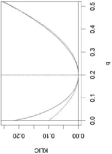
and if and only if . In Figure 3.1 an example is shown. It is assumed that . For comparison the dashed curve shows where a is chosen such that the the curves are close to the right of . It can be seen that KLIC acts much like quadratic distance to the right of the minimum, but has more curverture to the left.

Example of binary KLIC (solid line) compared to quadratic distance. It is assumed that q0 = 0.2.

Alignment methods.
We would like to minimize the information loss D given the restrictions (4), (5) and (6) from definition 1. The restriction (4) makes sure that we satisfy 1) in our list (ability to adjust correctly to the target means). The fact that we minimize the information loss satisfies 2) in the list (ability to retain the original shape of the probability distribution). ’Symmetric formulation’ and ’multinominal alignment’ follows automatically (point 4 and 5).
We can now derive our new alignment method:
Let (i = 1,…,N and a = 1,…,A) be the initial probabilities in a population. A Relative-Entropy-Minimizing Mean-Correction Alignment to a target is a set of aligned probabilities pia that minimize (14), given the restrictions (4), (5) and (6).
And we can prove the theorem:
Let p0 (i= 1,…,N and a= 1,…,A) be the initial probabilities in a population. In a Relative-Entropy-Minimizing Mean-Correction Alignment the aligned probabilities pia are given by:
where the parameters φa satisfy:
Proof. (White, 1982) Define the Lagrange-function L:
The first order derivatives are given by
such that:
Sum over the alternatives a(using (5)):
such that
Inserting this into (22) yields:
Observe that the Lagrange-parameters φa are not unique, as
We can therefore assume that
Observe that pia ∈[0,1] and that 3) is satisfied (retaining zero).
3.1 Logit scaling
We will actually prefere to give our method the catchier name Logit Scaling. The method fits perfectly a situation where the initial probabilities are supplied from a logit-model (point 6 in the list). Assume the probabilities are given by
where V0 are some logit-utilities. Then according to theorem 3:
The alignment is done by adding alternative-specific constants to the logit-utilities. As a corollary to this, if the preferences of the agents change in an additive way, the probabilities can be corrected with alignment. This is similar to the result in Li & O’Donoghue (2014) where it is shown that a “biased intercept” in a logit model can be corrected with some of the alignment methods (“Sidewalk hybrid with non linear adjustment” and “Sort by the difference between logistic adjusted predicted probability and random number”). Here we give a mathe- matical explanation.
After an alignment, the scaling parameters φa can be calculated and used to solve the following problem: assume we have a logit model describing some events in our microsimulation model. In the base run of the model we align these logit probabilities to given macro levels. In an alternative analysis we would like to calculate the behavioral responses using the logit model. But how can we do that when we have manipulated our logit probabilities in the alignment process?
Assume the logit model is given by
where x0 is a vector characterizing individual i and βa is a vector of logit-parameters for each alternative a. Let the aligned probabilities be:
Now assume we would like to analyze the effect of changing x0 to xi for all individuals i. Having calculated the φ!as we can calculate the new probabilities p^ia:
These probabilities will give the best possible representation of the marginal effects of the changed characteristics of the individuals.
If the aligned probabilities pia are known, it is possible to calculate the φ!as. It can be derived that, for any i:
This is so-called centered log-ratios known from compositional data analysis (Aitchison, 1986). Even if we are not doing the alignment via a direct calculation of the φ!as (an idea we will introduce in the next section) we can calculate them from (3.4).
In the binary case (A= 2) it can be proven that
such that the scaling factors are calculated from changes in log-odd-ratios.
3.2 An example
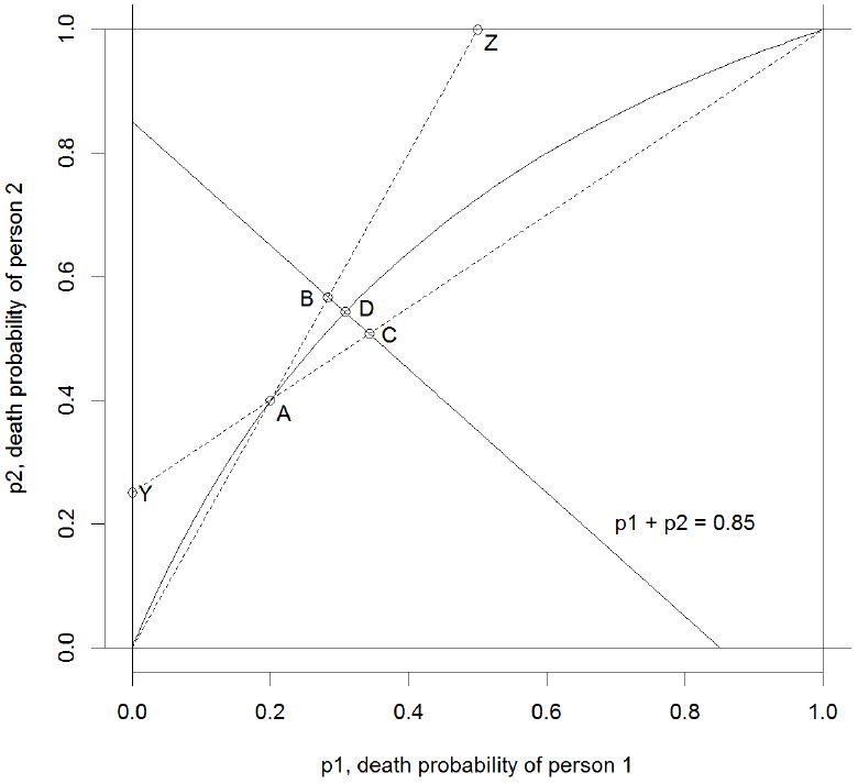
Let us consider a simple example. We have two alternatives (A = 2; death or survive) and two individuals (N = 2). We assume that the death probability of the first person is p1 = 0.2 (such that the probability of survival is 0.8) and the death probability of the second person is p2 = 0.4. The expected number of deaths in this tiny microsimulation model is 0.2 + 0.4 = 0.6. Let us assume we want to increase the expected number of deaths to 0.85. We will do this by alignment.
The first method we will use is the popular Multiplicative Scaling (Li & O’Donoghue, 2014). The initial point is A in the figure. The alignment process should move us to some point on the downward sloping curve defined by p1 + p2 = 0.85. With multiplicative scaling we have to possibilities4: scaling up the probabilities of death or scaling down the probabilities of survival. If we scale up the probabilities of death we move from A to B. If we scale down the probabilities of survival we move from A to C. As we can see there is a significant difference in the resulting alignments.
Another problem associated with multiplicative scaling is that the aligned probabilities can exceed 1. If the death probabilitis is scales up to a certain level we reach the point Z. Here the probability of death for person 2 is 1. Any further scaling will imply a death probability larger than 1. Likewise, if the probabilities of survival is scaled enough, we reach the point Y.
Now let us consider Logit Scaling. In the binary case we have from theorem 3 that:
The microsimulation model DYNACAN uses an algorithm called ’Sidewalk with Non-Linear Transformation’ (Li & O’Donoghue, 2014). This non-linear transformation is given by:
We can re-write (22) to:
such that the transformations are identical for
In the figure the solid non-linear curve shows all possible alignments for varying values of φ. The current align- ment is the point D. Observe that comparet to multiplicative scaling, the method is a compromise between point A and B. Also observe that the system can be aligned to any number of deaths between 0 and N = 2.
4. Bi-proportional scaling: An algorithmic solution
So far the alignment method seems to have nice theoretical properties, but how about the practical side of the equation? If we substitute the results of theorem 3 into equation (4), we get the following problem: choose parameters φa, a= 1,…,A, such that:
This is a system of Anon-linear equations with A unknowns. As A is typically small (2 to 10), this is not a big equation system. But from a computational point of view it is a problem that we sum over the number of individuals i. This can be a very big number (up to millions). We therefore need a fast algorithm.
The standard computational way to solve a set of non-linear equations is to use the Newton-Raphson algorithm. This algoritm works by making a local linear approximation of the system (the Jacobian mitrix). This linear system is solved (the Jacobian matrix is inverted), and by repeating the process it is possible to converge to the solution of the non-linear set of equations.
Using the Newton-Raphson algoritm implies the calculation of the A×A Jacobian matrix in each iteration, where each element in this matrix is a sum over all individuals. A considerably faster approach is Bi-proportional scaling. Look at the original problem: minimize (14) given (4) and (5). This is actually a Matrix Balancing Problem (Schneider & Zenios, 1990). Instead of the initial matrix P0 we should choose another matrix P, such that the difference between the matrices is as small as possible, and such that the row sums are given (see 2.2) and the column sums are given (see 2.1). It is well known (McDougall, 1999) that if the measure of difference between the matrices is Relative Entropy, then there exists a simple algorithm that converges to the solution of the matrix balancing problem. This algorithm is called bi-proportional scaling and is very simple and fast. You start out with the original matric P0. In this matrix the row sums are 1 because we work with probabilities. The column sums are equal to the expected numbers of outcomes distributed on the A alternatives. First you scale the columns such that the colums sums are correct according to the restrictions, i.e. the expected numbers are equal to the alignment targets. Then you scale the rows such that the column sums are correct (sums to 1 again). But then the column sums are not correct any more. If you repeat this process again and again, you will realize that the errors in the column sums will decrease dramatically, and the system will converge. In real world problems the convergence is very fast (often less than 10 iterations). We therefore have a very surprising result: our very non-linear problem can be solved by simpel iterative scaling.
The method is tested against two versions of the Newton-Raphson algorithm, a standard version and an op- timized version (see Table 1). The reason for this comparison is twofold: first, it is proven that Bi-proportional scaling is faster then the standard method (even when it is optimized), and second, it is demonstrated that the methods yields the same results.
Comparing Bi-proportional scaling with two Newton-Raphson algorithms (N = 1.000.000, A = 4). The centered log-ratios φas are the output of the Newton-Raphson algorithms. In the case of Bi-Proportional Scaling they are calculated using (3.4).
| Time (Sec.) | φ1 | φ2 | φ3 | |
| Newton-Raphson (Standard) | 3.94 | 0.53841805 | −0.58964392 | 0.00557946 |
| Newton-Raphson (Optimized) | 1.45 | 0.54167153 | −0.59175494 | 0.00659708 |
| Bi-Proportional Scaling | 0.60 | 0.53841807 | −0.58964390 | 0.00557951 |
In the standard version of the Newton-Raphson algoritm, the Jacobian matrix is calculated based on abstract differentiation of the non-linear equation system. In each iteration the elements in the matrix is calculated by an average over all individuals. The matrix is inverted using the C#-library Math.Net. In the optimized version, the procedure is the same except for the calculation of the Jacobian matrix. The elements in the matrix is averaged over a sample of 10 pct. of the individuals. This improves the speed, only slightly compromising precision.
The artificial population is 1.000.000 individuals with 4 alternatives. The artificial set of probabilities are cal- culated by drawing 1 mill. numbers from each of 4 normal distributions5. If (xi1,xi2,xi3,xi4) are these 4 number for individual i, the probabilitis are calculated as:
The result of the test is given in Table 1. Bi-proportional scaling ran twice as fast as the optimized Newton- Raphson, and more than 6 times faster than the standard Newton-Raphson. If we look at the centered log-ratios we see that these are practically identical for the standard Newton-Raphson and Bi-Propotional Scaling. As mentioned the speed of the optimized Newton-Raphson resulted in a somewhat lower precision. This precision cost is not observed for Bi-Proportional Scaling.
The final point on the list is ease of implementation. It took more than a week to develop and test the Newton- Raphson algorithms. When the idea came to the author, it took half an hour to code bi-proportional scaling, showing the power of the approach.
5. Conclusion
A general mathematical foundation of multinominal alignment in microsimulation models is derived. The alignment problem is characterized as the solution to an optimization problem. The analytical solution to this problem is characterized and applied in deriving various properties for the method. It is demonstrated that there exits an algorithm called Bi-Proportional Scaling that converges to the solution of the optimization problem, that the new method is more general than existing methods, and that it is fast and easy to implement.
Footnotes
1.
Or a more general term for both: moment correction, as it corrects the first two moments of the probability distribution.
2.
Admittedly this point is added because out method works well with logits.
3.
Q is actually a probability distribution as 0 ≤qia ≤1 and ), ), qia = 1.
4.
This asymmetry seems not to be a well-known in the microsimulation community. As an example it is not mentioned in Li & O’Donoghue (2014)
5.
The distibutions are: N(−3.0,0.8), N(−1.0,0.5), N(0,0.5) and N(−0.2,0.8) where the first number i mean and the second is variance.
References
- 1
-
2
Micro-macro linkage and the alignment of transition processes. Technical paper(25).Micro-macro linkage and the alignment of transition processes. Technical paper(25)..
-
3
The maximum entropy distribution of an asset inferred from option pricesJournal of Financial and Quantitative Analysis 31:143–159.
-
4
An information-theoretic alternative to generalized method of moments estimationEconometrica: Journal of the Econometric Society pp. 861–874.
-
5
Evaluating binary alignment methods in microsimulation modelsJournal of Artiftcial Societies and Social Simulation 17:15.
-
6
Entropy theory and RAS are friends. GTAP Working PapersEntropy theory and RAS are friends. GTAP Working Papers, 6.
- 7
-
8
A comparative study of algorithms for matrix balancingOperations research 38:439–455.
-
9
A simple nonparametric approach to derivative security valuationThe Journal of Finance 51:1633–1652.
-
10
Maximum likelihood estimation of misspecified modelsEconometrica: Journal of the Econometric Society pp. 1–25.
- 11
Article and author information
Author details
Acknowledgements
The author would like to thank Joao Miguel Ejarque, Michael Andersen, Marianne Frank Hansen and two anonymous referees for many thoughtful comments and edits. We would also like to thank the The Knowledge Centre for Housing Economics under Realdania for generous financial support.
Publication history
- Version of Record published: December 31, 2016 (version 1)
Copyright
© 2016, Stephensen et al.
This article is distributed under the terms of the Creative Commons Attribution License, which permits unrestricted use and redistribution provided that the original author and source are credited.