Projected population, inequality and social expenditures: The Case of Flanders
- KU Leuven, Belgium
- Vrije Universiteit Brussel, Belgium
Abstract
We investigate the budgetary and distributional effects of a demographic and economic evolution in Flanders between 2011 and 2031. We project demographic changes by means of two multi-state population projections (LIPRO-projections), on the basis of which we statically reweigh the EU-SILC 2008 dataset. In addition, we assume a modest real exogenous –meaning not induced by the demographic projections– growth rate of 1%. Population-wise, we find a pronounced ageing, a growth of single-headed households, mostly to the detriment of couples with children, and a closing generational gap in education. While income inequality exhibits a non-monotonous pattern over time (reaching a maximum around 2020), poverty steadily declines after 2011. We find a large increase in expenditures on pensions, which is, however, covered by the modest public income growth we assume, while keeping the tax system constant in real terms.
1. Introduction
Traditionally, in Flanders, household income is among the highest in Europe and inequality as well as poverty are low (Eurostat, 2014). Following the general trend in Western European countries, inequality declined between the 1950s up to the second half of the 1980s. Since then, however, there exists no unequivocal evidence for this equalizing tendency (Van den Bosch, Vandenbroucke, Cantillon, & Pacolet, 2009; Vranken, De Boyser, & Dierckx, 2006), except for Flanders where inequality remains consistently lower than in the rest of Belgium (Cantillon, Horemans, Vandenbroucke, & Van Lancker, 2011; FOD Economie, K.M.O., Middenstand en Energie, 2013).
In this paper, we extend the horizon of analysis, projecting income inequality and poverty indicators, as well as social expenditures for Flanders, up to the year 2031. Moreover, we analyse the underlying demographic elements affecting these evolutions. Traditionally, such trends were mainly attributed to economic factors, such as wages, income, or tax-benefit systems, (Bargain & Callan, 2010; Heathcote, Perri, & Violante, 2010); in contrast, we investigate the role of (projected) demographic evolutions as drivers of future income inequality and poverty trends.
The profound changes in Flanders’ population structure seem to justify our focus. In parallel with the well-documented ageing of the population (Federaal Planbureau en ADSEI, 2011; Studiecommissie voor de vergrijzing, 2006), the Flemish household composition changed quite substantially. From the 1960s onward, driven by new gender and generational relations, divorce rates started to rise, marriage became less popular and, with the exception of the baby-boom years, fertility continued to show an overall decreasing trend (Lesthaeghe & Neels, 2002; Van Bavel & Bastiaenssen, 2006). The onset of this so-called second demographic transition occurred about 20 years later in Belgium, particularly in Flanders, compared to neighbouring countries, while resulting trends were, until recently, less pronounced (Deboosere et al., 2009). After 1980, however, Flanders started to catch-up with international trends and different family formation processes proliferated. As a result, households have become smaller in general (Lodewijcks & Deboosere, 2011) and, especially among the young, unmarried couples and single-headed households have proliferated (Deboosere et al., 2009).
A second major evolution in the population structure concerns increasing educational achievement. Under the impulse of labour market demands and political and societal investments in the educational system, ever more children enter schooling and remain in training for a longer period of time (Vanderstraeten, 1999). Parallel, from the 1960s onward, we observe a democratization and growing gender equity in education, although social inequality remains a critical aspect of Flanders’ educational system at all levels (Pelleriaux, 2000; Verbergt, Cantillon, & Van den Bosch, 2009), the breach between classes has decreased (Groenez, 2010). Moreover, girls outperform boys at all educational levels for some time now (Pelleriaux, 2000). In short, since the 1960s, for each consecutive generation, educational levels are higher compared to earlier generations.
In recent literature, the importance of a clear understanding of the impact of population change on inequality and poverty has repeatedly been stressed (Blank, 1995, 2011; Burtless, 1999; Chen & Föster, 2011; Peichl, Pestel, & Schneider, 2012; Western, Bloome, & Percheski, 2008). This understanding is far from easy, since different components of demographic change are intertwined and may have counteracting effects. In this respect the ageing, in particular the growing share of the population above 65, is presumed to increase inequality, since elderly population’s income is lower and their poverty ratio higher than that of the working-age population. In addition, in Flanders, this generational gap seems to have increased over time (Van den Bosch et al., 2009). However, ageing also implies an increase in life expectancy, and couple’s survival has a positive effect on household income: women depend less on a widows’ pension and also, with the increase in education and female labour force participation, households will often have two pensions or combine a pension with (the younger womans’) income from wages. Consequently, the net effect of ageing on the income distribution remains ambiguous. Mookherjee and Shorrocks (1982) found that, in the UK, the shift in age-income relationship had an impact on inequality, but the population’s compositional change did not. More recently, the latter was confirmed for other European countries by the Social Situation Monitor (European Commission: DG Employment, Social Affairs & Inclusion, 2017).
On the basis of all 22 countries present in the Luxembourg Income Survey, it has been shown (Tai & Treas, 2008, 2009) that, even in the case of single-headed households, the effects on inequality are not clear-cut. Being less able to pool income resources (combined with the gender pay gap), single-headed households and especially single parents have a lower income compared to the household income of the rest of the population. In addition, no improvement in the situation of single parents is observed over time (Tai & Treas, 2008, 2009). This general phenomenon is also observed in Flanders (Studiedienst Vlaamse Regering, 2013; Van den Bosch et al., 2009). A rise in the prevalence of female single-headed households is therefore often found to trigger an increase in inequality and poverty (Bradley, Huber, Moller, Nielson, & Stephens, 2003; Kollmeyer, 2013). With the increase in education and subsequent increased female labour force participation, however, this tendency might reverse. In addition, Esping-Andersen (2007) indicates that the negative influence of single motherhood is mainly restricted to the United States as the strong European welfare state mitigates its impact.
The rise in educational attainment and the concomitant increase in female labour force participation is also found to increase inequality since double-income households are concentrated at the top of the income distribution (Esping-Andersen, 2007). However, the larger the group of the educated and the lower educational disparity, the smaller the role this factor will play in the determination of income inequality. In the long run, we might well expect the rise in educational attainment to temper inequality. In this respect, Breen and Salazar (2010) found that changes in women’s education and their behavioural consequences account for little if any of the growth in earnings inequality between households, while Kollmeyer (2013) found that it decreases inequality.
This work joins a strand of recent research aiming at quantifying the role of demographic change on inequality (Peichl et al., 2012), but in contrast to former studies, we analyse this relationship prospectively, focusing on the 20 year period from 2011 to 2031. From a policy point of view, this is important; for social policy to go beyond ad hoc answers to structural changes, it needs to be informed on how future population (and economic) characteristics affect inequality. In addition, this prospective view can re-mediate some of the difficulties related to contextual factors faced by retrospective research (Esping-Andersen, 2007). Building on hypothetical scenarios about economic growth and population forecasts, we isolate our analysis from temporal and contextual influences and gain at least partial control over interactions with non-observed variables. Note that we limit our attention to the coming 13 year period, which is the time frame in which the baby-boom generation will reach retirement age. Moreover, beyond this time frame, predictions become increasingly uncertain.
The prospective nature of our endeavour firmly roots it in the microsimulation tradition. A microsimulation model (MSM) is essentially a forecasting device that simulates aggregate and distributional effects of change –such as population change– by applying it to a representative sample of individuals or families, subsequently adding up the results across individual units using population weights (Bourguignon & Spadaro, 2006; Martini & Trivellato, 1997). The results in this paper were obtained using the microsimulation model Mefisto.1 The baseline model used in this paper investigates the effect of demographic change under the condition of a 1% economic growth attributed to efficiency increases.2
To disentangle economic from demographic growth, we use two decomposition methods. The first is based on the construction of a counterfactual, which involves reweighing the sample at t0 such that the distribution of population covariate levels becomes identical to the sample at t1. Comparison of the counterfactual Gini-index with the actual one at t0 reveals the effect of changing population structure, while the difference between counterfactual and the distribution at t1 is a residual effect. This method is known as the Blinder-Oaxaca decomposition (Blinder, 1973; Oaxaca, 1973). In the context of distributional analysis it has been applied by DiNardo, Fortin, and Lemieux (1996), Hyslop and Maré (2005), Handcock and Morris (1998), Bargain and Callan (2010), to name but a few. The second method concerns an exact decomposition of the inequality index (Shorrocks, 1980, 1984) to gain insight into the influence on inequality and poverty of shifts in population subgroup prevalences.
In Section 2 we describe the data and methodology. Section 3 presents the results of the population projections. Section 4 describes the forecasted income inequality evolution and its relation to demographic and economic change, with Subsection 4.3 focusing on budgetary effects.
2. Methodology
We proceed with a number of distinct steps:
We first make multi-state demographic projections at five-year intervals for twenty years (from 2011 up to 2031) by age, sex and household position and by age, sex and educational attainment. The procedure is described in Subsection 2.2.
We calibrate the EU-SILC 2008 data to the distribution of the different population subgroups obtained by the demographic projections. In other words, we reweigh the EU-SILC 2008 in such a way that the income data match the population forecast obtained in step 1. This procedure is called static ageing (see Subsection 2.3).
We choose a realistic scenario for economic growth to update the income data in EU-SILC 2008 for each five-year interval from 2011 to 2031 (as described in Subsection 2.4).
Finally, based on the re-weighted and uprated income data obtained from steps 2 and 3, we estimate inequality and poverty indices, as well as the budgetary implications for each five-year interval (details can be found in Subsection 2.5).
2.1 Data
The population as found in the 2001 Belgian census data served as the baseline for the population projections. The 2001 Census data were linked to the National Register data, using the individual’s unique National Number. This provided the information on transitions in household positions and in educational attainment levels during a period of five years. In addition, births, deaths and migratory movements were extracted from the same data sources.3
The EU-Statistics on Income and Living Conditions (EU-SILC) database is our main source of information on income, social inclusion and living conditions. In addition, data on housing, labour, education and health are collected as well.4 Information on household position is not available as such, but is extracted from the relationships of parenthood and partnership between all household members. This procedure is explained in the Appendix. At the start of this research, the microsimulation model Mefisto ran on the EU-SILC 2008 dataset, which explains our choice for that particular cross-section.
2.2 Multi-state population projections
We used the LIPRO (Lifestyle Projection) Method as proposed by Van Imhoff and Keilman (1991), for which the 2001 Census data provided the baseline population. For the projection by household position, the population is broken down by five-year age groups, sex and 12 “LIPRO household positions”: children of married and unmarried couples, children in lone parent households, married and unmarried couples with or without children, single households, lone parents, non-related family members, members of collective households and a residual category.5 For the projection by educational attainment level, the state vector comprised of five-year age groups, sex and nine educational levels: individuals are either still in school or have finished school attaining one of the following levels: primary education, lower secondary education (general, technical and professional), higher secondary education (general, technical and professional) or higher education.
LIPRO-projections estimate population structures prospectively by multiplying the density of the initially observed population state vector (baseline vector) with a transition matrix to obtain the density of the state vector in the next period. We thus estimate two first-order Markov models: the first has a state vector consisting of age groups, gender and household position. The second first-order Markov model has a state vector consisting of age groups, gender and educational attainment level.
This way the population is recursively projected one period ahead. The transition rate matrix indicates the probability to transit from one household position (educational level) to another. The matrix also includes death and emigration rates from each household position (educational level) as well as births and immigration to each household position (educational level). The initial transition rate matrix is estimated from the linked 2001 Census data and National Register Data and refers to the transition probabilities between 1 January 2001 and 1 January 2006 .6
For consecutive five year projection periods up to 2026–2031, the transition rate matrix is adapted using scenarios based on prognoses about the evolution of fertility, mortality and migration (Studiedienst Vlaamse Regering, 2011). We assume that the recent revival of fertility in Flanders will continue up to the period 2016–2021, while going down again afterwards (Schockaert & Surkyn, 2012). Life expectancy is expected to continually increase, a little faster for men than for women. In addition, we assume that international immigration increases up to the 2016–2021 period and remains constant at that level thereafter. Emmigration increases linearly with about 20% over the whole projection period. The combination of both hypotheses results in the pattern summarized in Table 1. Note that we assume that the household formation processes will remain identical during the complete projection horizon. This means that the forecasted population structure and its impact on inequality and expenditures are the result of the ageing and the projection of household formation processes of the current population. In the case of the educational projection, we assume a slight rise in educational retention.7
Projection scenarios.
| Period | ||||||
|---|---|---|---|---|---|---|
| 2006–10 | 2011–15 | 2016–20 | 2021–25 | 2026–30 | ||
| Fertility (births per woman) | 1.73 | 1.82 | 1.76 | 1.72 | 1.70 | |
| Life expectancy (years) | Female | 82.7 | 83.2 | 83.8 | 84.4 | 85.0 |
| Male | 76.9 | 77.7 | 78.7 | 79.6 | 80.7 | |
| Net migration (rate/base rate) | 1 | 1.2 | 1.4 | 1.2 | 1 | |
| Educat. retent. (rate/base rate) | 1 | 1.065 | 1.13 | 1.195 | 1.25 | |
The LIPRO-projection model presents some clear advantages with respect to classical projections by age and sex only. First, the results are much richer. Secondly, LIPRO is a fully dynamic model where vital events and migration are differentiated by, and interact with household formation or educational processes. If, for example, fertility is lower among higher educated women, a rise in the population’s educational levels will temper total fertility rates, even though for all educational levels alike we considered a relative fertility increase comparable to the one predicted by Studiedienst Vlaamse Regering (2011). In other words, important compositional population changes mitigate the evolution of fertility, mortality and migration, and consequently impose constraints on future population trends. Thirdly, modification in one household position also imposes constraints on the adjustments in other household positions. For example, if for the purpose of population projections we accept the number of same-sex couple formation to be negligible, the number of men that transit into the state of “married couple without children” should be equal to the number of women entering this state (and vice versa). In other words, LIPRO calibrates the theoretically linked transitions. The constraints included in the household projection are explained by Schockaert and Surkyn (2013). For the educational projection, no constraints were used. The above properties of LIPRO projections enhance the reliability of the results by ensuring coherence in population trends.
2.3 Static ageing and calibration to obtain household weights
An overview of weighting methods can be found in Kalton and Flores-Cervantes (2003), keeping in mind that most of these methods were conceived to re-mediate survey non-response (Holt & Elliot, 1991). Reweighing by a simple reweighing of cells (Kalton & Flores-Cervantes, 2003), however, is ruled out for two reasons. First, due to insufficient observations we use two sets of demographic projections. Since these are made independently from each other, they possibly result in conflicting reweighing factors. Although a simple solution seems to be available by calibrating the conflicting individual weights, a second more fundamental problem remains. In the described demographic projections, the unit of observation is the individual, while for our distributional analysis, we prefer the household as unit of observation, since the household composition is the cornerstone for equivalising income. In order to marry the individual-based demographic projections with the household-based inequality and poverty analysis, we calibrate the base year sample using household weights to the individual-based totals implied by the demographic projections (Deville & Sarndal, 1992). Such a calibration procedure finds new weights as close as possible to the old ones, such that the individual-based demographically projected totals are respected.8 A detailed description can be found in De Blander, Schockaert, Decoster, and Deboosere (2013).
2.4 Economic growth
In order to obtain a realistic impression of future (equivalised) income distributions and concepts derived thereof, such as inequality and poverty, not only demographic changes need to be taken into account, but we need to make some assumptions concerning economic growth as well.
Clearly, economic growth is not independent of demographic changes. It can be split up into the following components:
An increase in workforce participation rate. We assumed that this component remains unchanged, conditional on the variables used in the demographic projection, that is sex, age, household position and education. Any changes in this component are thus mainly driven by ageing and educational changes.
Productivity growth, which breaks down into two components:
an endogenous productivity growth component, caused by the changing distribution of individual and household characteristics over time (considering the projections we use, the main source of this component is an increase in educational attainment). Whenever a (projected) population stabilizes, this component tends to zero. Keep in mind that we assume that the returns to education remain at their present level.
an efficiency growth component, conditional on individual and household characteristics, induced by the fact that, people produce ever more, hence more efficiently, without any change to said characteristics, including hours worked.
Since changes in workforce participation rate and endogenous productivity growth are completely determined by the demographic projections, we name the sum of both the demographic growth. It is only the varying component of productivity growth, conditional on the demographic assumptions, for which we need to make additional assumptions, and which we termed efficiency growth. In the remainder of this paper, we assume that the efficiency growth amounts to a yearly real-term increase of 1%.9
Following additional assumptions are made:
economic growth is proportionally shared among the factors of production, which entails that (self-)employment income and income from capital have the same growth rate.
benefits grow according to the assumptions described in Dekkers, Desmet, Fasquelle, and Weemaes (2013): the minimum income will grow at an annual rate of 1% in real terms, all other benefits at 0.5%.
To ensure that we do not overestimate inequality, we allow pensions to grow with the efficiency growth rate. Let us justify the pension growth rate by providing an example. Consider a pensioner in the observed sample who retired five years prior to observation at time t0. In the philosophy of the reweighing methodology, this observation will represent a number of pensioners at time t1, who will have retired in t1 − 5. Exact calculation of their pension would involve calculating each observation’s last wage at t0 − 5, applying the observed real wage growth between t0 − 5 and t0, applying the hypothesized real wage growth between t0 and t1 − 5, and finally, applying an hypothesized real pension growth between t1 − 5 and t1. Simply up-rating pensions by the hypothesized real wage growth rate will produce accurate results if:
real pension growth rates between t1 − 5 and t1 are identical to those between t0 − 5 and t0,
the real wage growth rate between t0 − 5 and t0 was close to the hypothesized real wage growth rate.
It seems reasonable to make assumptions concerning incomes in terms of the efficiency growth rate, since collective wage agreements pertain to individual increases in wages. Assuming the educational attainment of one firm, or even a whole sector of the economy, remains quite stable over time, wage increases will be accorded conditional on age and education of employees. Likewise, an increase in benefits is stated as a percentage increase of the individual’s benefit. Consequently, wage and benefit rises seem not directly connected with any demographic evolution. The demographic growth component is not observed by individual firms, but only appears ex-post at the aggregate level.
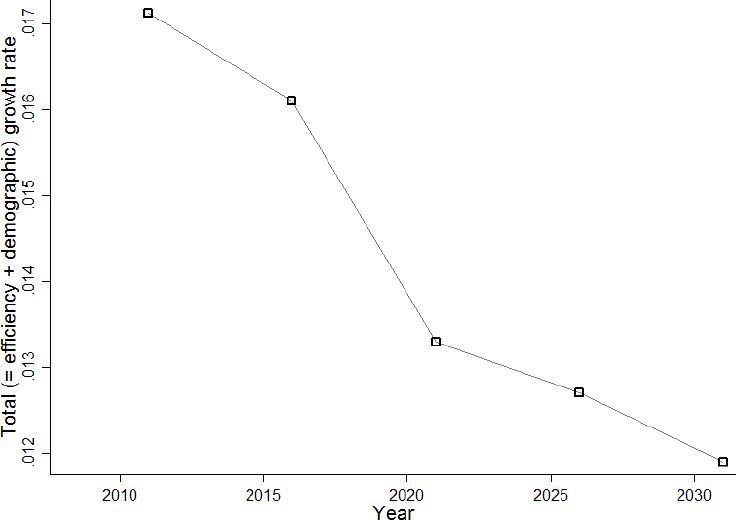
The resulting factors by which incomes and pensions are uprated can be found in Table 2. As mentioned above, this represents only the efficiency growth component of the total economic growth, the second component arising from the fact that increasingly educated cohorts grow older. The combined effect of efficiency growth and growth induced by demographic change is depicted in Figure 1. It is obtained by calculating the growth rate of aggregated primary income per capita, under the combined demographic and economic assumptions, which should be a close proxy to projected per capita economic growth. The total growth rate gradually decreases to the annual efficiency growth rate of 1%. Although this boundary is not fully reached, the projected evolution is consistent with what we theoretically expect: once we reach a stable population (keeping boundary conditions on fertility, migration,... constant), economic growth will settle at the level of what we termed the efficiency growth component.
Up-rate factors.
| year | factor |
|---|---|
| 2011 | 1.030 |
| 2016 | 1.083 |
| 2021 | 1.138 |
| 2026 | 1.196 |
| 2031 | 1.257 |

The macro-economic growth rate resulting from both effciency and demographic growth.
As small word of caution might be in order: the endogenous productivity growth component is driven by the fact that younger cohorts are more educated, leading to an increasing educational average over time. Our results partly depend on one of the many implicit ceteris paribus assumptions we have made: the returns to education remain fixed at their present level. However, the returns to education can fluctuate for each education level depending on the relative demand and supply in each labour market segment. Jobs for which there are shortages of qualified candidates, will typically be more highly remunerated. On the other hand, if the proportion of highly educated increases faster than the labour demand for this type of workers, we might witness a decrease of the return to education over time for the highest educated. Such a detailed level of labour market scenarios is, however, beyond the scope of this paper.
2.5 Measuring inequality and poverty
In this Subsection, we describe the way inequality and poverty will be measured, keeping in mind that, under the assumptions we made, everybody improves in absolute and real terms.
2.5.1 Inequality indexes
We calculate two inequality indices: the Gini coefficient and the Theil index. For some continuous (income) distribution F with mean μF, the Gini coefficient is formally defined by
where the variable x represents an equivalised net income of an individual i. In this paper, we use the OECD equivalence scale, which gives full weight to the first household member, 0.5 to subsequent adults and 0.3 to each child. The value of the Gini coefficient ranges from 0 at complete income equality (everybody earns the same amount) to 1 when inequality is maximal (only one individual earns total income). If we only have a sample at our disposal, the Gini coefficient can be estimated by
with xi representing a realization of x.
The Theil index is a competing inequality measure.10 It is given by
It ranges from 0 at complete income equality (everybody earns the same amount) to ln N, when inequality is maximal (only one individual earns total income). It is measured by
The main advantage of the Theil index is its sub-group decomposability, that is
where g= 1,..., G constitutes a partition11 of the population, qg is the equivalised income share of subgroup g, TFg is the Theil index of sub-group g and TB is the between group Theil index. It is calculated by attributing every individual the group-mean equivalised income μFg.
In the context of our study, this property of the Theil index is helpful: it allows analysing the contribution of specific changes in the prevalence of population categories, for example, the increase of single-headed households or individuals with higher education, to the forecasted changes in inequality. The largest part of this contribution originates from the second part of the formula
In order to assess the difference in Theil index, ΔTF , between two periods, t1 and t2, we decompose its difference in a Blinder-Oaxaca fashion as
where
2.5.2 Poverty
Foster, Greer, and Thorbecke (1984) introduced the family of poverty indices
known as the Foster-Greer-Thorbecke class of poverty measures, where x represents equivalised net household income, f(x) its density function and with z the poverty line or poverty threshold. In this paper, we use a relative poverty line, defined as 60% of the median equivalised income of the Flemish population. Note that the poverty line varies over time. PFGT (F|z, 1) is the normalized poverty gap. The (non-normalized) poverty gap per poor person is equal to the difference between the individual’s income and the poverty line divided by the poverty rate. It is an indicator of the severity of poverty.
A key advantage of the FGT class of poverty indices is its subgroup decomposability, that is
with pk the population share belonging to subgroup k and Fk the income distribution within subgroup k. As in the case of the Theil decomposition, we will use the poverty decomposition to gain insight in the impact of specific shifts in the population composition on poverty.
Similar to inequality, we decompose differences in a poverty index, [triangle]PFGT (F|z, α), between two periods, t1 and t2, in a standpoint-neutral (Reimers, 1983) Blinder-Oaxaca fashion as
The difference in poverty index can thus be seen to originate from a compositional effect
3. Demographic trends
During the second half of the last century, intense modifications in family formation and dissolution were observed (Deboosere et al., 2009): a postponement of first marriage, a reduction of marriage intensity and an increment in divorce rates. These evolutions, in combination with the endurance of fertility decline and the increase of life expectancy, will induce a profound change in Flanders demographic structure over the next twenty years.
Figure 2 shows the population distribution by age and sex in 2011 and the projection result for 2031. As the baby-boom generations at working and reproductive age in 2011 grow older, the bottom of the pyramid shrinks and the top becomes heavier. Parallel, this ageing process gives rise to changes in the population’s household composition as the younger generations of 2011 grow older and their family formation behaviour is reflected in successive age groups in each subsequent projection year. This is demonstrated in Figures 3–5.
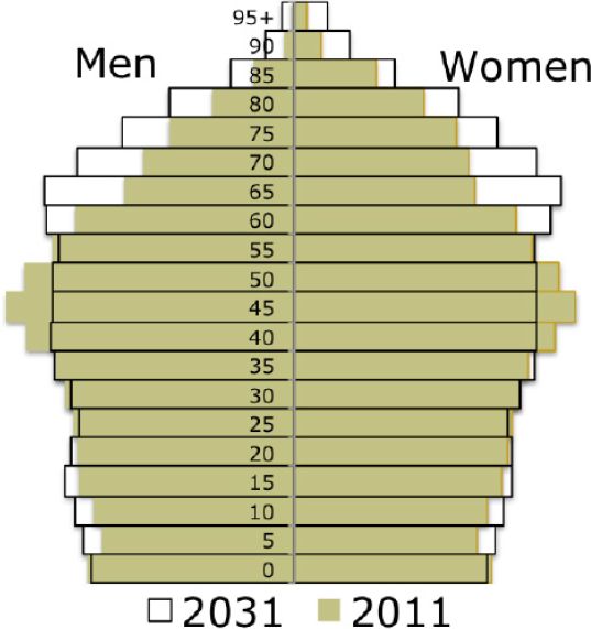
Population pyramid 2011 – 2031.
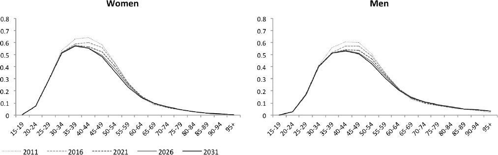
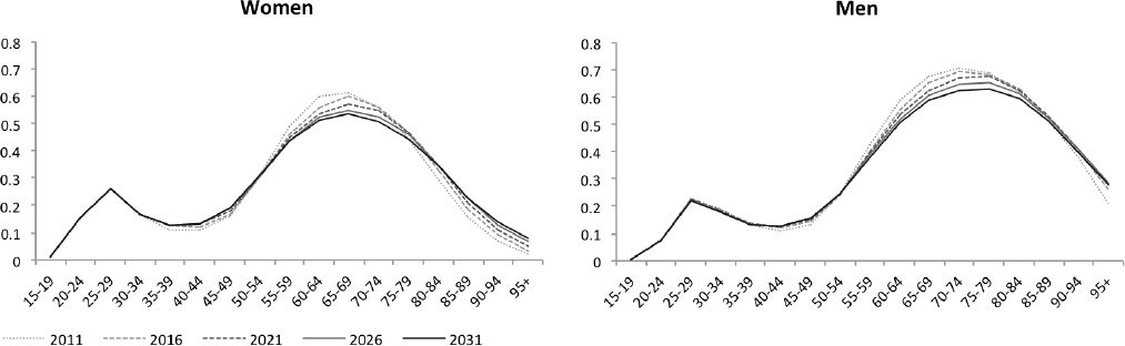
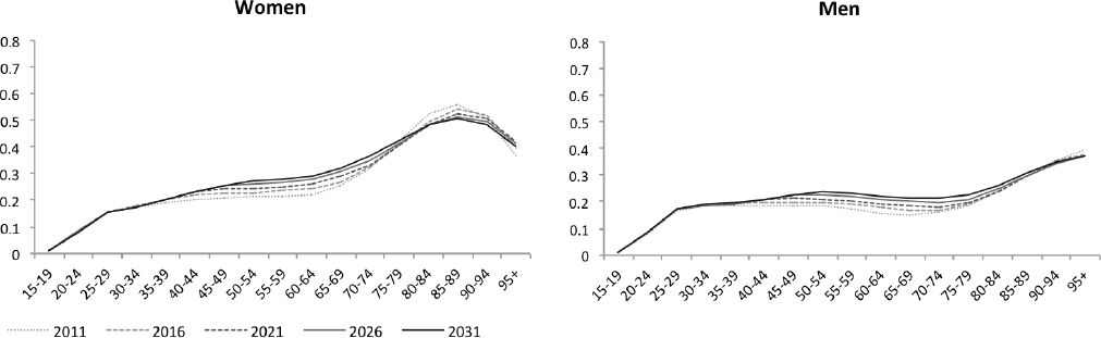
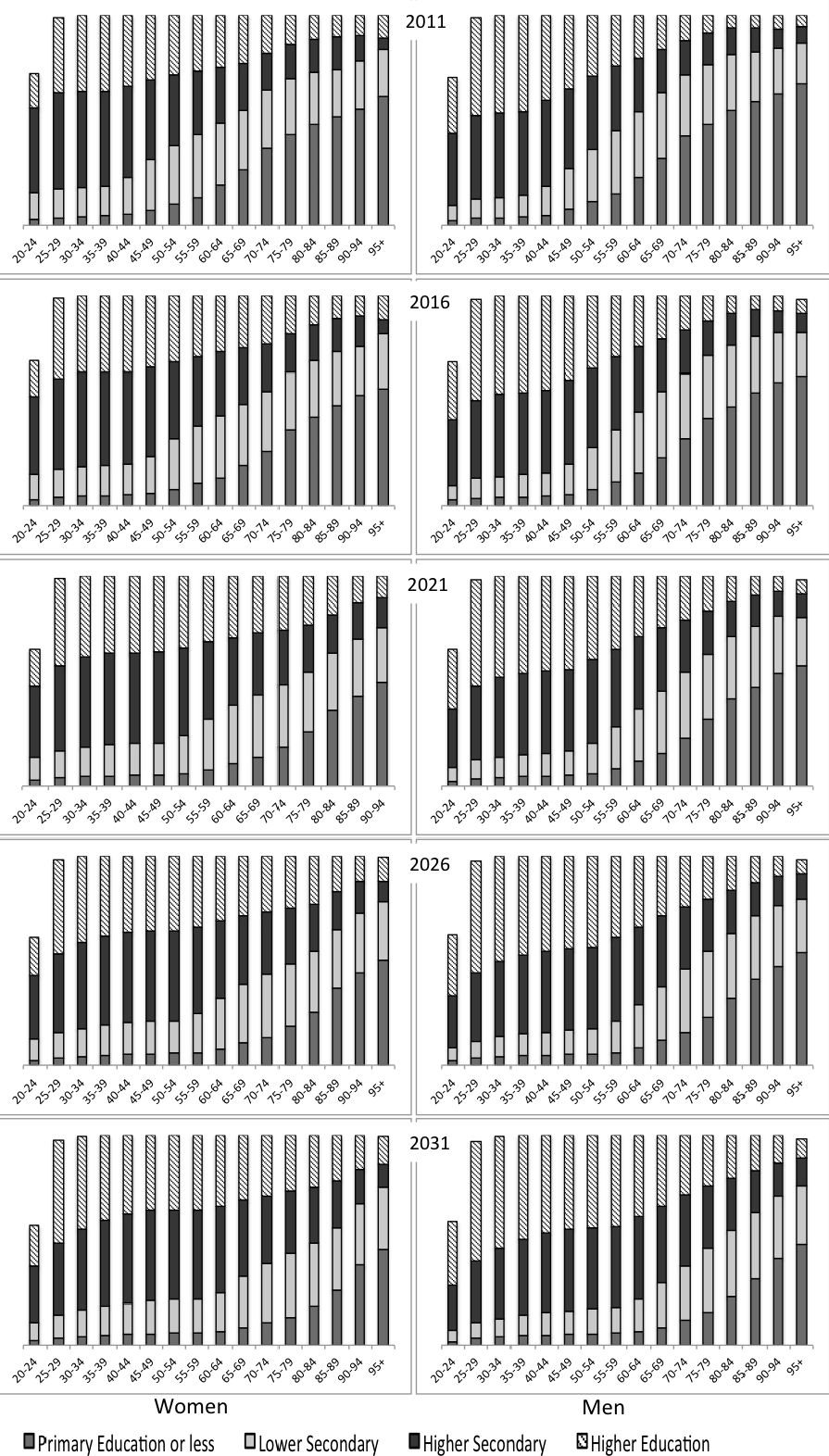
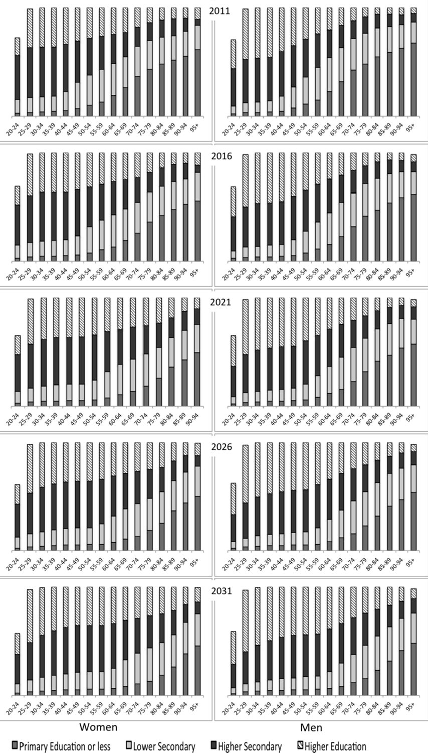
Figures 3–5 depict the proportional distribution of household positions, by age for each five-year projection period between 2011 and 2031. The x-axes represent five-year age groups and the y-axes, the proportion of individuals from each age group in single-headed households (Figure 5) and in couples with and without children (Figures 3 and 4, respectively). Each curve, from light to dark grey, represents a consecutive projection year. A first important evolution is the decrease of the share of individuals that live in couples with children. This is related to the decrease and postponement of couple formation and to fertility decline. The latter development explains the larger decrease after the age of 40, as low fertility leads to a shorter total time span that children are present at their parent’s household. Higher divorce rates add to this evolution and also explain the decreasing prevalence of couples without children at more advanced adult age. However, among the elderly population, above the age of 75 for women and 85 for men, the prevalence of individuals living in a couple increases in time. This is easily understood as the result of growing partner’s survival rates since we projected women’s and especially men’s life expectancy to grow. The decrease in the share of couples in the population over time results in the rise of single-headed households, most eminent between the age of 40 and 70.

Couples with children by age and sex.

Couples without children by age and sex.

Single-headed household-heads by age and sex.
Figure 6 depicts the proportional distribution by age of individuals with only primary or less education, lower and higher secondary education and higher education for each five year projection period between 2011 and 2031, for women (left panels) and men (right panels). The Figure shows that parallel to ageing and changes in household position, for all age groups and each gender, we foresee a considerable advancement in educational attainment. That is, for each age group the share of the population with higher secondary and higher education becomes larger over time. This process is almost entirely due to the ageing of the population as from each projection year to the next, the educational profile of the younger generations is progressively spread to all ages. Therefore, in the first part of the projection period, especially the 40 − 64-age group’s educational attainment increases; in the second half of the projection period, the 65+ educational attainment rises most while below 60, practically no change is observed any more. Within the population under the age of 35, practically no change is observed since we assumed only minor adaptations in educational behaviour (see Table 1). Consequently, in the long run, an equalizing tendency between generations and gender is observed.
The following comparison demonstrates this tendency: in 2011, the part of the population having at least a higher secondary degree below the age of 40 was about 80% while this was only the case for about 22% of the group above 65. In 2031, 80% of the whole population under 65 will have a higher secondary degree, and this is also the case for almost 60% of the 65+ group. Furthermore, in 2011, the younger generations of women had already exceeded the education level of men; in 2031 this will be the case for all age groups, except the most advanced ones.
4. Inequality and poverty effects
4.1 Demographic and efficiency growth effects on inequality and poverty evolutions
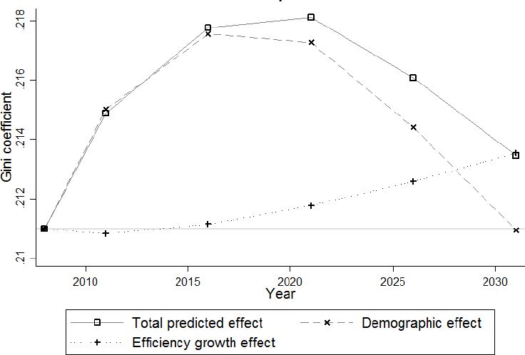
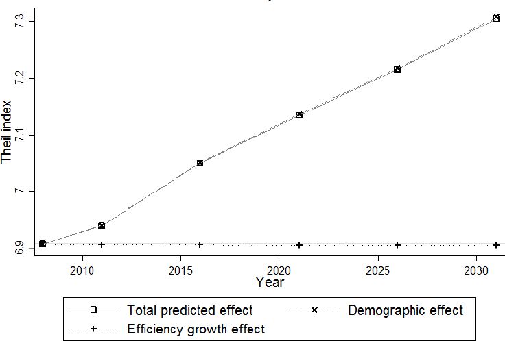
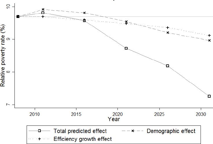
In this Section we depict the forecasted change in income distribution, using the Gini (1) and Theil (3) indexes for describing the overall inequality changes. In addition, the poverty rate and poverty gap (Figures 9–11) focus on the evolution of the lower tail of the income distribution. The curves called “total predicted effect” trace the evolution of each indicator when we carry out projections as described in Section 2. Note that the interpretation of such a curve should be comparable to the year 2008, represented by a horizontal grey line.
We decompose this projection into its constituent components, following the Blinder-Oaxaca decomposition method of Section 1. The efficiency growth effect is obtained by keeping the population identical to its 2008 distribution, while attributing every individual an income increase as described in Subsection 2.4. The “demographic effect” results from the projected evolution in population composition, but keeping real incomes constant at their 2008 level. Note that the total effect is not always the sum of the two partial effects, as interaction induces some degree of non-linearity.
Both the temporal evolution and the decomposition into a demographic and an efficiency growth effect of the Gini and the Theil indices are similar (see Figures 7–8). The overall inequality change is mainly driven by the population component with a rather small efficiency growth effect added to it.
Population and educational attainment by age and sex.

Inequality measure: Gini coefficient.

Inequality measure: Theil index.
Inequality peaks around 2021 and reaches a level comparable to 2008 in 2031. Note however that the predicted change is quite small. At its peak in 2021, the Gini coefficient has only increased 0.007 points in absolute terms (which corresponds with roughly 3%) above its initial level of 0.211. Of this change, about 86% is due to demographic changes and only 14% to the efficiency growth effect. However, in 2031, the Gini coefficient is only 0.002 points (1%) above its initial level, with 100% of the increase explained by the efficiency growth effect.12 The Theil index follows a similar pattern, with a maximal increase of 0.008 points (9%). While the efficiency growth effect increases inequality due to the different growth rates between gross wages and the different types of benefits, we refer to Subsection 4.2 for a detailed analysis of the effect of demographic changes on inequality.
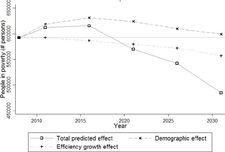
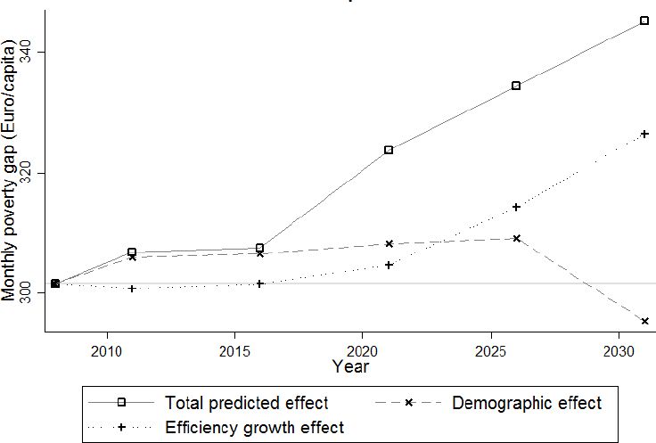
Figure 9 depicts the projection of the relative poverty rate. From 2011 onward, both indicators steadily decrease from a maximum of about 13.5% and 10% to 11.5% and 7.3% respectively. The number of people in poverty (Figure 10) follows a similar pattern. This is the result of the efficiency growth effect, reinforced after 2016 by a demographic effect.13 In contrast with the poverty rate, the average poverty gap (Figure 11) systematically increases from 300 € to about 340 €. In other words, despite the decrease in poverty risk, for those in poverty, the situation becomes more severe.

Relative poverty rate.

People in poverty.
Monthly poverty gap per poor household.
In short, inequality rises during the first decade of the projection period and decreases afterwards. Poverty also increases, but for a shorter period of time. Furthermore, overall inequality changes seem mostly driven by demographic factors, while the poverty evolution in addition strongly depends on the forecasted economic factors.
4.2 Understanding the effect of population change
Up till now, we established the effect of the joint forecasted population changes and compared them with the efficiency growth effects. In this Section, we break down “demographic effect” of Figure 8 and Figure 9 in order to gain insight into the way population change affects inequality and poverty. Some shifts in the prevalence of particular sub-groups described in Section 3 give some suggestions, but evolutions are intertwined and/or imply contradictory effects, rendering straightforward and simple predictions quite hard.
Let us first take the example of ageing. On the one hand, ageing implies an increase of the population above the age of 65, which consists frequently of pensioners with an income below average. On the other hand, ageing also implies an increase in life expectancy, and the longer survival of a couple has a positive effect on household income. As a consequence: women will depend less on a widows’ pension in 2031. In addition, with the increase in female education and labour force participation, households will more often have two pensions at their disposal or combine a pension with (the younger woman’s) income from wages. Consequently, the net effect of ageing on the income distribution is a priori unclear.
The decomposition method for the Theil index was explained in Equation (5) of Subsection 2.5; the decomposition of the poverty index was presented in 9 of Subsection 2.5. To isolate population change, we keep the individual wages constant to those of the base year 2008 (“no efficiency growth”). Students and age groups below 25, over-represented among students, are excluded from the analysis. Since their household income is directly linked to that of their parents, they don’t properly contribute to shifts in income distribution or poverty.
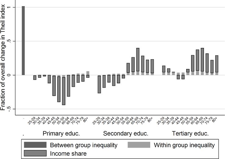
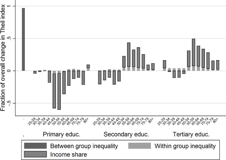
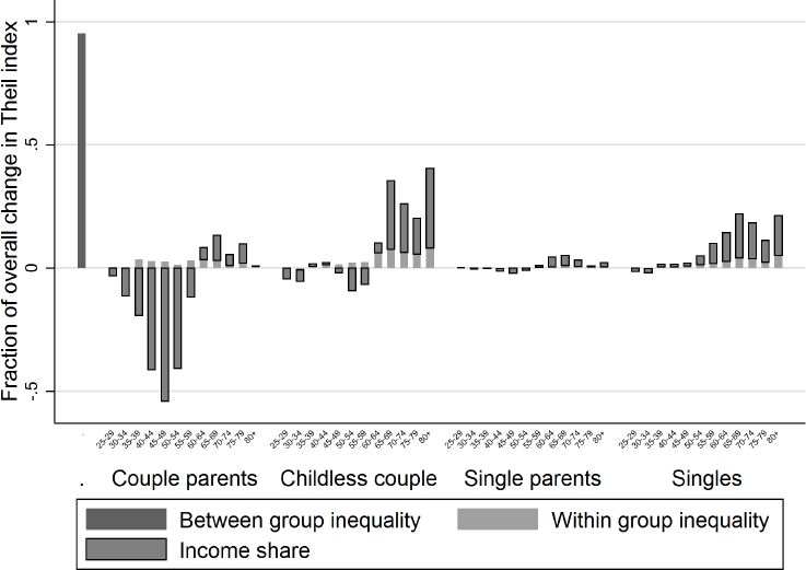
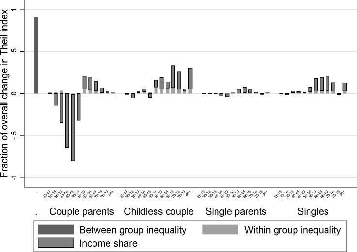
Figures 12–13 show the decomposition of the change in Theil index (as given in Figure 8) due to changes in age distribution and educational levels. Figures 14–15 show the decomposition due to changes in age distribution and household position. Figures 12 and 14 analyse the overall inequality reduction between the beginning and the end of the projection period (2011 versus 2031). Figures 13 and 15 are restricted to the period of temporal inequality increase between 2011 and 2021.

Decomposition of the change in Theil index with respect to sub-populations by age and educational attainment, period 2011–2031.

Decomposition of the change in Theil index with respect to sub-populations by age and educational attainment, period 2011–2021.

Decomposition of the change in Theil index with respect to sub-populations by age and household position, period 2011–2031.
The first bar at the left depicts the change in the between-groups Theil index. The other bars indicate the contribution of changes in each population subgroup to the total inequality change. The size of the bar indicates the size of contribution to inequality change; upward means a positive impact, downward a negative one. As became clear from Equation (5), the subgroup contribution depends on the inequality evolution within the group and the group’s share of the total population’s income, represented in light and dark grey bars respectively. Note that both effects are entirely due to population change, since we assume “no efficiency growth”. Clearly, changes in the income shares are largely driven by observed changes in the population composition; a change in the prevalence of a population category provokes an income share change in the same direction. This way we can directly link the results with the population change described in Section 3. Changes in the within-group inequality are related to the subgroup composition with respect to the demographic variables omitted in the decomposition exercise (sex and household composition in the first and sex and education in the second exercise), but that induce changes in the subgroup’s labour force participation rate and/or endogenous income growth.
Figure 12 indicates that the overall decrease in inequality between 2011 and 2031 is due to a reduction of between-group inequality and to the decrease in income share of the population with no or only primary education. The latter process is related to the general increase in educational attainment depicted in Figure 6. The reduction of between-group inequality can easily be understood by the attenuation of generational differences in education. However, Figure 12 also shows that the increase of the income share of individuals over 55 with secondary or higher education, increases inequality. In other words, ageing and the subsequent growth of the elderly population increases inequality, despite their higher educational attainment. This effect is nonetheless insufficient to offset the overall inequality decrease.
During the first part of the projection period between 2011 and 2021, in contrast, the impact of ageing does outgrow that of educational attainment growth effect and between-group inequality reduction, as shown in Figure 13. Consequently, Figure 8 showed an increase of inequality between 2011 and 2021.
Figures 14–15, decomposing the Theil index by age and household position, also reveal that the growth of the elderly population’s income share positively contributes to the Theil index, whether living as a couple or in single-headed households. The decrease of the adult population younger than 55 living in couples with children has a negative impact on inequality. Note that the within-group inequality among many couples of the same age group increases, as well as the between-group inequality between 2011 and 2021. This can be explained by the fact that educational growth, especially at the beginning of the projection period, increasingly differentiates among individuals in similar household positions. This process is more evident in couples than single-headed households due to the larger effect of education on the income growth of double-income households.14

Decomposition of the change in Theil index with respect to sub-populations by age and household position, period 2011–2021.
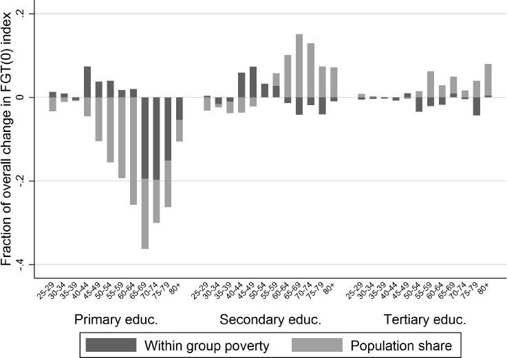
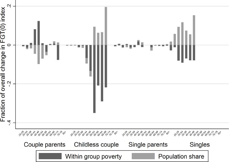
Figures 16–17 show the decomposition of the declining poverty trend between 2011 and 2031 (see Figure 9). Figure 16 refers to the decomposition by age and educational attainment; Figure 17 to the decomposition by household position. The bars indicate each population group’s contribution to the overall poverty change, depending on the within-group poverty and the population share of each group, represented in light and dark grey bars respectively (see Equation (5)). The size of the bars indicates the size of contribution to inequality change; upward means a positive impact, downward a negative one.

Decomposition of poverty change by age and educational attainment.

Decomposition of poverty change by age and household position.
Figure 16 shows that the poverty decrease between 2011 and 2031 is largely due to the decrease of the population share with only or less than primary education . This effect is somewhat attenuated at more advanced ages due to the ageing of the population, but it is completely compensated by a prominent reduction in the poverty levels among the group above the age of 65. Among secondary and higher educational levels, the effect of ageing takes the upper-hand; the increase of the population share above the age 55 increases poverty, despite the increased educational levels. Moreover, among the adult population between the ages 35 and 60, we even observe an increase in within-poverty due to educational change
Figure 17 shows that, both the growing population share of single-headed households among the lower income groups and the diminishing population share of couples without children among the higher income groups, have an increasing effect on poverty. However, the reduction of poverty levels most pronounced for childless couples, but also witnessed for single-headed households counteracts to this effect sufficiently to account for the poverty reduction witnessed between 2011 and 2031. This indicates that the educational increase is most concentrated among individuals living in these types of household (for instance childless couples and single-headed households). The contribution of changes in couples with children is rather modest; their increased prevalence (see Figures 3–5) leads to a modest negative effect on poverty, compensated by an increase in within-group poverty levels.
4.3 Budgetary effects
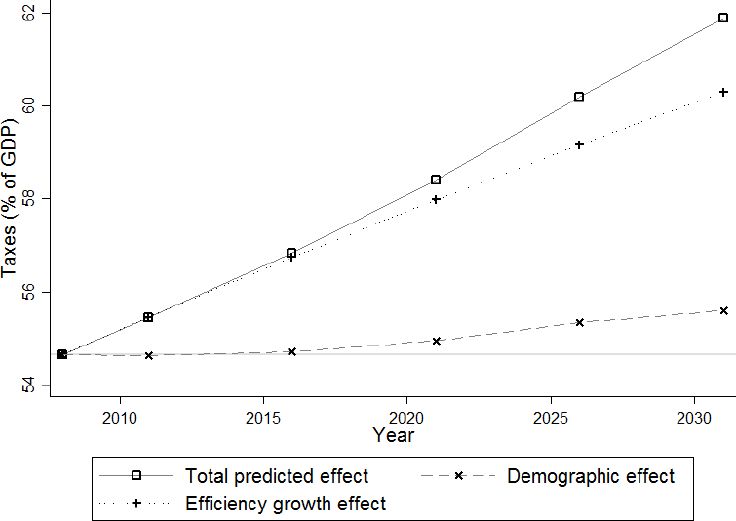
In Figures 18–20 we present the projected evolution of payments made to all levels of government and benefits received from all levels of government by Flemish households, expressed as a percentage of aggregated gross incomes. These numbers are generated by the MSM Mefisto, which models the Belgian tax-benefit system. We decompose the “total predicted effect” into an efficiency growth effect, by increasing each individual’s income, keeping the population structure identical to the 2008 structure, and a “population effect”, by changing the population structure to match the population forecasts, but keeping constant individuals’ income in real terms (see Section 4).

Evolution of income taxes and social security contributions as a percentage of total income.

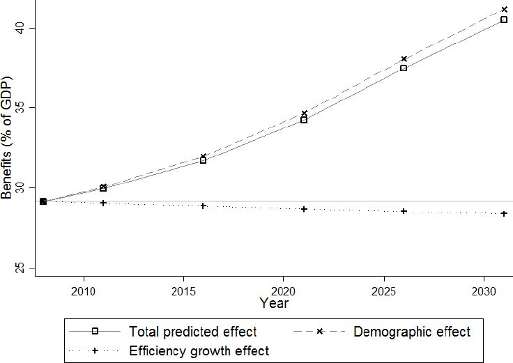
Evolution of all social security payments received as a percentage of total income.

Net yearly payments made.
Figure 18 depicts the total direct payments made by Flemish households to all levels of government (that is federal, regional and local). These payments consist of income taxes and social security contributions. Demographic changes have only a moderate effect on the total direct payments, increasing them by around 1% –from 54.5% to 55.5%– between 2008 and 2031, again in percentage of aggregated gross income. In contrast, the efficiency growth effect induces an almost linear increase in taxes from 54.5% in 2008 to 62% in 2031. This tax increase is mainly caused by increasing real wages in a progressive tax system assumed to be constant in real terms, that is a tax system where the brackets are only indexed with inflation, resulting in an increasing real average tax rate.
The evolution of the total predicted effect climbs slightly above the efficiency growth effect. Note that, in general, the total effect, measured as the difference between a given point in time and year 2008, is not always the sum of the two partial effects, measured similarly, but a sometimes quite important interaction effect induces some degree of non-linearity. For example, the difference between the total predicted effect on taxes in 2031 and the horizontal line marking the level of taxes in 2008, is larger than the sum of the demographic and the efficiency growth effects in Figure 18.
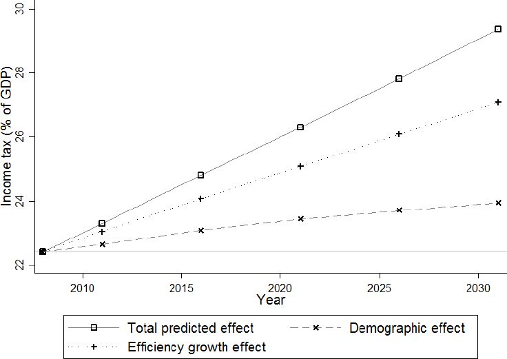
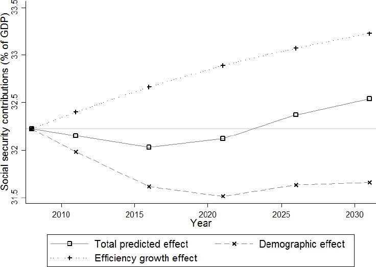
The total tax burden is broken down into its constituent components: income tax (Figure 21) and social security contributions (Figure 22). Income tax is predicted to rise almost linearly from 22.5% of total gross income in 2008 to 29% in 2031. About two thirds of its increase are induced by the efficiency growth effect, while the remaining one third follows mainly from the endogenous growth due to increasing educational levels. Social security contributions fall below their initial level of 32.2% of total gross income until 2021, but climb to 32.5% in 2031. This last evolution is the combined effect of a linearly increasing efficiency growth effect with a negative demographic effect, which stabilizes around –0.7% after 2021.
Evolution of income taxes.

Evolution of social security contributions.
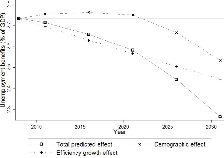
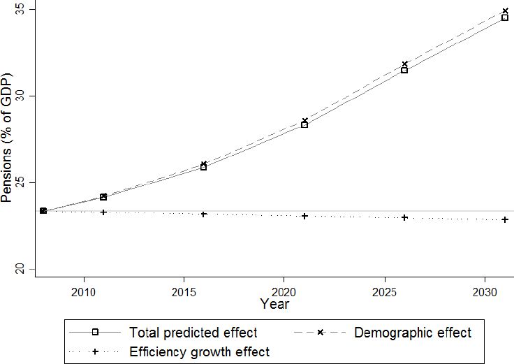
In Figure 19, the dependent variable is the sum of child benefits, minimum guaranteed income, unemployment benefits and pensions (again expressed as a percentage of aggregated gross incomes). While the efficiency growth effect on total received benefits decreases by about 1%, the total increase from 29% to 40% is mainly driven by the demographic effect. Breaking down all benefits received into their four components (Figures 23–26), the bulk (80% of total benefits) consists of pensions, with the remainder about equally divided between child (10.3%) and unemployment benefits (9.4%) in 2008. In 2031, however, the share of pensions has increased to 85% of total benefits at the expense of the unemployment benefits (6%), and with child benefits slightly decreasing to 9% of total benefits.
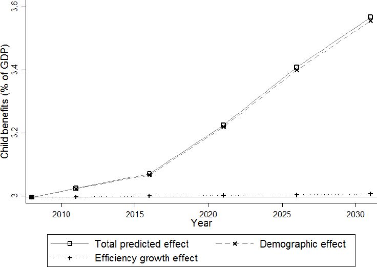
Evolution of different types of child support.
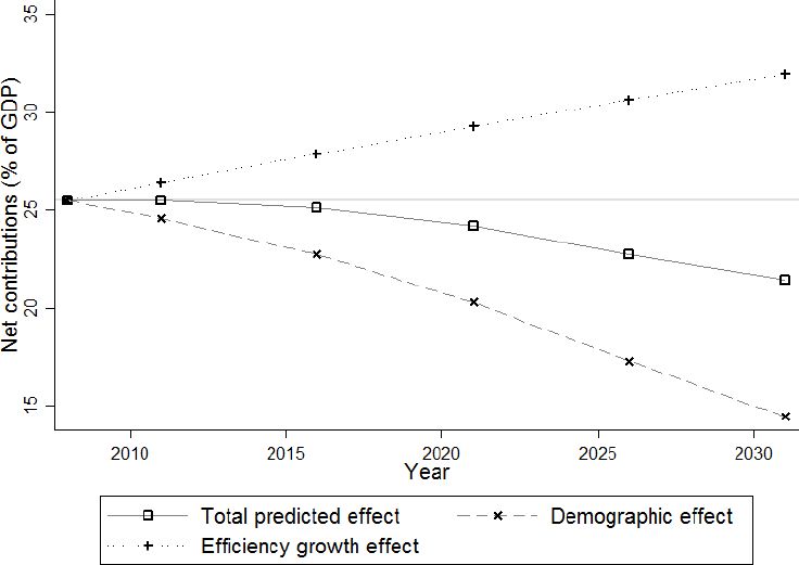
The difference between Figures 18 and 19, is given in Figure 20. It could be considered as a measure of the size of government pur sang, meaning that part of revenues which is not redistributed right away. Here the two partial effects oppose each other, resulting in a steady decrease of the total effect from 25% to 20%. Remarkably, the total predicted size of government expenses, expressed per capita (instead of relating it to total gross income) is roughly the same in 2031 as in 2008. This means that the non-redistributive tasks of the aggregated government, such as law enforcement, infrastructure, education and health care, for example, can remain at their 2008 level, in real terms, per capita. In other words, under the assumed growth scenario and keeping the tax-benefit system constant in real terms, in twenty years time the aggregated collective sector governing the Flemish population will be able to provide the same level of services and collective goods per capita as today, despite the increasing share of pensions in total income from 23% in 2008 to 34% in 2031 (see Figure 26).
Note that when we consider the social security system separately, and compare benefits received (Figure 19) with contributions made (Figure 22), the surplus of about 3% (32.25% contributions paid by households obtained from Figure 22 minus 29.25% benefits received by households obtained from Figure 19) in 2008, is turned into a deficit of 6.5% (32.5% contributions paid minus 39% benefits received) in 2031 (all quantities measured as percentage of aggregate gross income). This in turn could have lead us raise alarmist warnings about the sustainability of pensions. Indeed, in a steady state, that is, a state without any demographical or other transition, any system can only be sustainable if it complies to a budget constraint. In this respect, two remarks are in order:
The ageing of the population is a transitory effect, hence any ceteris paribus steady state reasoning seems a priori overly simplistic.
Notice the use of the word system, without the “social security” qualifier.
Indeed, when considering the complete collective sector, that is the combined government and social security revenues, our exercise shows that the increased income taxes ensuing from only a moderate exogenous growth, will easily pay for the increased volume of pensions, while at the same time leaving everyone better off (at a growth rate of 1%) in real terms, compared to the present situation. This seemingly counter-intuitive conclusion is explained by two phenomena:
fiscal drag: keeping the fiscal system constant (in real terms) generates super-linear incomes (in real terms) for the government.
consolidation of government functions: by not artificially separating redistribution from consumptive public expenditures, we allow the fiscal drag to pay for the baby-boom ripple.
As the population approaches a new steady state, the fraction of taxes needed to subsidize the social security system can be brought down again, albeit to a higher level as before, due to the higher life expectancy.
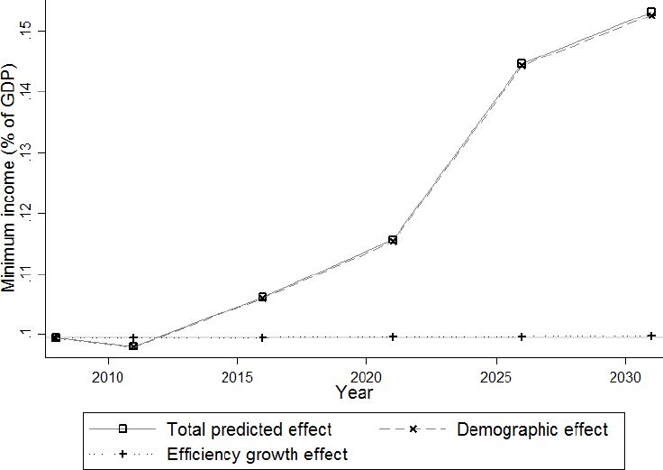

Evolution of minimum income.

Evolution of Unemployment benefits.

Evolution of Pensions.
5. Conclusions
In this paper, we forecasted changes in inequality, poverty and social expenditures in Flanders between 2011 and 2031, and analysed their relationship to population change. We used multi-state population projections (LIPRO-projections) based on Census and Register data from 2001 and 2006. We reweighed the EU-SILC 2008 survey data to construct the necessary income data for each five year period between 2011 and 2031. Assumptions about population change were conservative: we presumed only changes in mortality, fertility and migration following the current official Flemish hypotheses, whereas household formation processes and educational behaviour were kept (nearly) constant to the projection base-year information of 2006. In addition, we assumed a modest economic efficiency growth of 1% annually.
Our population projections foresee a pronounced ageing of the Flemish population between 2011 and 2031. Along with the ageing process, characteristics of the current younger generations are spread to older age groups. Consequently, the projection results demonstrate an increase of single-headed households to the detriment of couples, especially those with children. Educational attainment levels increase and intergenerational and gender differences attenuate.
Under the assumptions mentioned, inequality and poverty show unequal forecasted evolutions and are differently affected by demographic and economic change. Inequality, measured by the Gini and Theil indices, is lower in 2031 than in 2011, but it exhibits a non-monotonous pattern over time, reaching a maximum around 2020. This pattern is mainly driven by population change, while economic growth has a small but increasing impact over time. Poverty steadily declines from 2011 onward. This is due to a growth effect, reinforced by population change.
The evolution of public finances is forecasted as follows. On the revenue side, income taxes increase from 22% to almost 30% of gross income earned by all families. On the expense side, pensions increase from 23% to 34% of gross income earned by all families. However, this spectacular increase in pension volume is completely paid by the modest growth we assume and by keeping the tax system constant in real terms. These results are obtained without altering the retirement age, nor the real level of pensions.
In order to gain insight into the relationship between population and inequality change, we decomposed the Theil index and the poverty rate into the effects of shifts in particular subgroups defined by age and household composition on the one hand, and age and educational level on the other. The impact on inequality of changes in population subgroups remain similar over time, but depending on the observation period the effect of one predominates over the other. In addition, the results show the counteracting effects of the population ageing process. With ageing, the elderly population increases but educational levels also rise and generational differences attenuate. Over the total observation period between 2011 and 2031 the latter two processes play the larger role: the overall decrease in inequality is mainly due to a declining between-group income variation reinforced by a decline of the population with no or only primary education. Also the drop in prevalence of couples with children reduces inequality. During the period between 2011 and 2021, in contrast, the impact of the growing elderly population, especially single-headed households, outgrows that of educational attainment growth and between-group inequality reduction, producing a temporary increase in inequality. The reduction in poverty between 2011 and 2031 can to a large extent be attributed to the decrease of the population share with only or less than primary education. Among the elderly population this effect is enhanced by a a prominent reduction in within-poverty levels. Educational increase counterbalances the effect of the rise of single-headed households to the detriment of couples, that would have increased overall poverty if their poverty levels would not have declined due to educational improvement.
Footnotes
1.
MEFISTO is a tax-benefit simulator based on the Euromod architecture, incorporating indirect taxes and specific Flemish policy responsibilities.
2.
See Subsection 2.4 for a decomposition of economic growth and more explanation.
3.
A detailed description of this procedure can be found in Schockaert and Surkyn (2012).
4.
The Council and European Parliament regulation 1177/2003 and subsequent documents, provide its legal and technical framework.
5.
The application of the LIPRO-household typology to the Census and register data was discussed intensively by Deboosere et al. (2009) and will be omitted in the current paper.
6.
A detailed description of the projection by household position can be found in Schockaert and Surkyn (2012).
7.
Retention refers to the share of the students that stay in education from one year to the next, and consequently, obtain a higher educational degree.
8.
The calibration was performed using the reweight command from Stata, contributed by Pacifico (2014).
9.
A quick survey of the World Bank website (World Bank, 2017) informed us that the average GDP growth rate for Belgium amounted to 2.64% (1960–2016), 1.53% (2000–2016) and 1.07% (2007–2016). We let the reader decide whether our choice is conservative or too optimistic.
10.
It is a member of the class of generalized entropy measures.
11.
is a set of subgroups, such that every individual belongs to exactly one subgroup
12.
Compare this with the results of Blank (2011, ch.4, p.94), who only attributes a mere 15% of the 1979–2007 rise in the US Gini coefficient for total income to demographic changes.
13.
Note that the joint effect is larger than the sum of the demographic and efficiency growth effect, indicating an important interaction between both evolutions.
14.
Assortative mating and it’s effects on income inequality is well-documented (Greenwood, Guner, Kocharkov, & Santos, 2014; Schwartz, 2010).
Appendix
Constructing a LIPRO-typology for EU-SILC
The first step of the reweighing procedure consists of knowing for each individual, its age, sex and household position. The former two variables are readily available in the EU-SILC; household position however is not. In this Section we explain how we constructed a LIPRO household typology within the EU-SILC dataset. The EU-SILC questionnaire identifies the relationships of parenthood and partnership between all household members. Figure A.I shows an extract of the Belgian EU-SILC questionnaire on the relationships among household members. Based on information directly from the National Register, in column 2 and 3, the names of each household member are printed. In column 2I to 24, the interviewer enters the line number (column I) corresponding to the father, mother, spouse or partner of each individual.

The EU-SILC questionnaire on relationships among household members.
Notes: Note that “voorgedrukt” and “voorg” means that the information is taken directly from the National Register. The interviewer only verifies it. Source: National Register of Belgium.
To assign a LIPRO household position to each individual in the database, we started with the basic rules presented in Table A.1. In the case of nuclear families, the application of the above rules is not problematic. In the case of extended families, additional restrictions become necessary. When the extended family involves grandparents, parents and children, the grandparents are assigned the MAR+ or UNM+ category. This implies that the second generation is classified as CMAR or CUNM and the grandchildren will be OTHR/NFR. The same rule is applied if there is only one grandparent present; the first generation is H1[a80]A, the second C1[a80]A and the grandchildren OTHR/NFR. This choice has implications for the population structure. Most grandparents are married couples, while this is less the case for the second generation among which consensual unions are more accepted. If we had the MAR+ of UNM+ categories to the second generation, more individuals would have been UNM+.
To verify the compatibility of the EU-SILC LIPRO typology and the Census typology, we compare the population structure by age, sex and household position in EU-SILC (2008) and in the results of the population projection. The continuous lines in represent the distribution by age, sex and LIPRO-household position for 2008 resulting from the weighted average of the 2006 Register data used in the projection and the projected population for 2011. The dotted lines show the distribution from the EU-SILC data, taking into account the original weights. Since both distributions refer to the same population, they should be identical. However, we observe some important discrepancies. In the case of children’s household positions, the population distribution by age and sex in EU-SILC closely follows the one of the Projection (Figure A.2). There are a little less C1PA children of young age and slightly more CUNM children in EU-SILC. Also the proportion of singles (SING) and lone parents (H1PA) seems to be slightly underestimated in the EU-SILC with respect to the projection, while the part of married men and women with or without children (MAR0 and MAR+) is somewhat higher (Figure A.3).
Rules for creating a LIPRO-typology in EU-SILC.
| SING | only individual living in the household |
| H1PA | someone’s parent and without partner |
| MAR0 | married with partner and not someone’s parent |
| MAR+ | married with partner and is someone’s parent |
| UNM0 | someone’s partner (one of both unmarried) and not someone’s parent |
| UNM+ | someone’s partner (one of both unmarried) and someone’s parent |
| CMAR | has a parent with a partner, both are married |
| CUNM | has a parent with a partner, one of both is unmarried currently married |
| C1PA | has a parent without partner |
| OTHR or NFR | All other positions |
| COLL | Collective households are excluded from EU-SILC |

Comparison of the population distribution by age and sex in EU-SILC and the projection, SING, MAR0, MAR+.
The largest difference however is found among the UNM0 and UNM+ categories for which the EU-SILC shows a considerable larger part of the young adult population. Several processes are at the basis of these divergences. The underestimation of singles, and single parents and their children in the EUSILC most probably reveals a sampling error not entirely corrected by the weights; drop-out and non-response is higher among individuals living alone (or alone with children) than among larger households. The larger proportion of UNM0 and UNM+ in EU-SILC than in the Projection Results is more puzzling. In the Census and Register data used for the projections, the LIPRO-household position is defined using the relationship of each member with the household head. While in the EU-SILC data, the unmarried couple is always defined as UNM0 or UNM+, this is not the case in the Projection Results, where another member can take the role of the household head. More important yet is the absence of a clear manner to identify consensual unions in Census and Register data; when the household head is not married, no relationship is defined. To identify the UNM0 and UNM+ individuals, Deboosere et al. (2009) therefore proposed that individuals of the opposite sex and without family relation to the household head are a potential partner. However, this person should have an age difference of at least 15 years to all other non-family related members. This last restriction may lead to an underestimation of consensual unions.
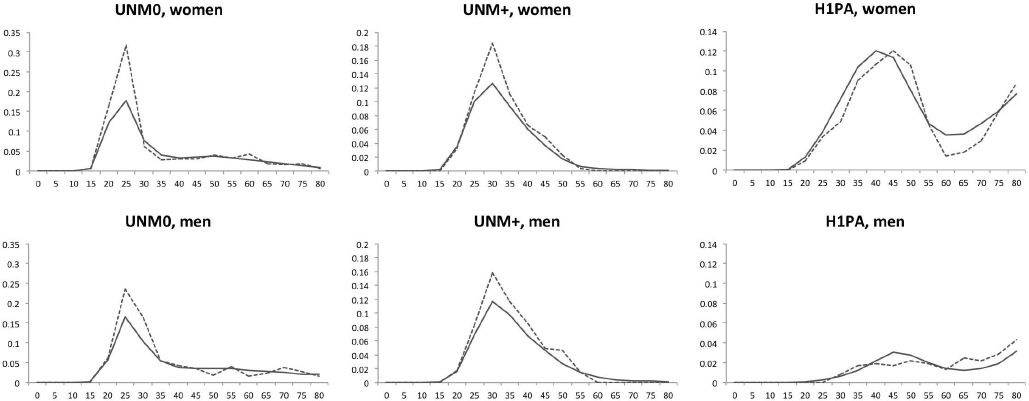

Comparison of the population distribution by age and sex in EU-SILC and the projection, UNM0, UNM+, H1PA.
References
-
1
Analysing the effects of tax-benefit reforms on income distribution: A decomposition approachJournal of Economic Inequality 8:1–21.
-
2
Changes in inequality and unemployment over the 1980s: Comparative cross-national responsesJournal of Population Economics 8:1–21.
- 3
-
4
Wage discrimination: Reduced form and structural estimatesJournal of Human Resources 8:436–455.
-
5
Microsimulation as a tool for evaluating redistribution policiesJournal of Economic Inequality 4:77–106.
-
6
Distribution and redistribution in postindustrial democraciesWorld Politics 55:193–228.
-
7
Has increased women’s educational attainment led to greater earnings inequality in the United Kingdom? A multivariate decomposition analysisEuropean Sociological Review 26:143–157.
-
8
Effects of growing wage disparities and changing family composition on the U.S. income distributionEuropean Economic Review 43:853–865.
-
9
Inkomen en armoede in Vlaanderen en Europa131–160, Eds., De sociale staat van Vlaanderen 2011, Studiedienst Vlaamse Regering, http://www.deverenigdeverenigingen.be/images/stories/SSV_2011-publicatie.pdf.
-
10
http://www.bmask.gv.at/cms/site/.../0/7/.../oecd_divided_we_stand_2011.pdfDivided we stand: Why inequalities keep rising.
-
11
The impact of demographic change on policy indicators and reforms (FLEMOSI Discussion Paper No. DP25)CES - KU Leuven.
-
12
http://statbel.fgov.be/nl/binaries/mono_200104_nl[1]_tcm325-92942.pdfHuishoudens en gezinnen in België (No. 4).
-
13
The social and budgetary impacts of recent social security reform in Belgium. Technical ReportThe social and budgetary impacts of recent social security reform in Belgium. Technical Report, Federal Planning Bureau, Belgium, https://lirias.kuleuven.be/bitstream/123456789/442606/4/Dekkers_Desmet_Fasquelle_Weemaes_impactofreform_IMA_2013.pdf, Paper presented at the IMPALLA-ESPANET International Conference“Building blocks for an inclusive society: empirical evidence from social policy research”, Luxembourg, April 18–19, 2013.
-
14
Calibration estimators in survey samplingJournal of The American Statistical Association 87:376–382.
-
15
Labor market institutions and the distribution of wages, 1973-1992: A semiparametric approachEconometrica 64:1001–1044.
-
16
Sociological explanations of changing income distributionsAmerican Behavioral Scientist 50:639–658.
-
17
website. Retrieved fromResearch findings – social situation monitor – decomposition of inequality by population subgroups, website. Retrieved from, http://ec.europa.eu/social/main.jsp?catId=1050&intPageId=1882&langId=e.
-
18
http://epp.eurostat.ec.europa.eu/portal/page/portal/income_social_inclusion_living_conditions/legislationRegulation (EC) 1177/2003 of the European parliament and of the council concerning community statistics on income and living conditions (EU-SILC).
- 19
-
20
http://www.plan.be/admin/ uploaded/201112190816070.bevpop2011_nl.pdfBevolkingsvooruitzichten 2010-2060 (Vooruitzichten).
- 21
- 22
-
23
Marry your like: Assortative mating and income inequalityAmerican Economic Review 104:348–533.
-
24
Onderwijsexpansie en – democratisering in VlaanderenTijdschrift Sociologie 3–4:199–238.
- 25
-
26
Unequal we stand: An empirical analysis of economic inequality in the United States, 1967-200615–51, Review of Economic Dynamics, 13, 1, Special issue: Cross-Sectional Facts for Macroeconomists.
-
27
Methods of weighting for unit non-response333–342, Journal of the Royal Statistical Society. Series D (The Statistician), 40, 3, Special Issue: Survey Design, Methodology and Analysis, 2.
-
28
Understanding New Zealand’s changing income distribution, 1983-1998: A semi-parametric analysisEconomica 72:469–495.
- 29
-
30
Family structure, female employment, and national income inequality: A cross-national study of 16 Western countriesEuropean Sociological Review 29:816–827.
-
31
From the first to the second demographic transition: An interpretation of the spatial continuity of demographic innovation in France, Belgium and SwitzerlandEuropean Journal of Population 18:325–360.
-
32
Households and families: Stability and fast development go hand in hand (GGP Belgium Paper Series No. 6)Households and families: Stability and fast development go hand in hand (GGP Belgium Paper Series No. 6), Generations & Gender Programme Belgium, GGP Belgium Paper Series - No. 6. Retrieved from, http://www.ggps.be/doc/GGP_Belgium_Paper_Series_6-EN.pdf.
-
33
The role of survey data in microsimulation models for social policy analysisLabour 11:83–112.
-
34
A decomposition analysis of the trend in UK income inequalityEconomic Journal 92:886–902.
-
35
Male-female wage differentials in urban labor marketsInternational Economic Review 14:693–709.
-
36
sreweight: A Stata command to reweight survey data to external totalsStata Journal 14:4–21.
-
37
Does size matter? the impact of changes in household structure on income distribution in GermanyReview of Income & Wealth 58:118–141.
-
38
(TOR Working Paper 2000/41)Het ontstaan van een demotiecultuur in het secundair onderwijs. een cultuursociologische analyse van de nieuwe vormen van ongelijkheid en van de nieuwe sociale kwestie, Doctoral dissertation, Vrije Universiteit Brussel, Faculteit Economsiche, Sociale en Politieke Wetenschappen, Vakgroep Sociologie, Onderzoeksgroep TOR, Brussels, http://www.vub.ac.be/TOR/cgi-bin/publicatiea.cgi?Command=Opzoeken&opdracht=auteur&id=11, (TOR Working Paper 2000/41).
-
39
Labor market discrimination against hispanic and black menReview of Economics and Statistics 65:570–579.
-
40
Snapshots of our future families (FLEMOSI Discussion Paper No. 12). VUBSnapshots of our future families (FLEMOSI Discussion Paper No. 12). VUB, http://www.flemosi.be/uploads/125/FLEMOSIDP12PopulationProjectionbyHH.pdf.
-
41
Technical report on the LiPro-projections (FLEMOSI Working Paper). VUBTechnical report on the LiPro-projections (FLEMOSI Working Paper). VUB.
-
42
Earnings inequality and the changing association between spouses’ earnings1524–1557, American Journal of Sociology, 115, 5, doi: 10.1086/651373.
- 43
- 44
-
45
http://www.plan.be/admin/uploaded/200611090953120.OPVERG200601nl.pdfJaarlijks verslag (Tech. Rep.). Hoge Raad van Financiёn.
-
46
SVR-internet page. Retrieved fromSVR-projecties van de bevolking en de huishoudens voor Vlaamse steden en gemeenten, 2009–2030 (Tech. Rep.), Brussels, Studiedienst Vlaamse Regering, SVR-internet page. Retrieved from, http://data.gov.be/nl/dataset/svr-projecties-van-de-bevolking-en-de-huishoudens-voor-vlaamse-steden-en-gemeenten-2009-2030.
-
47
http://ebl.vlaanderen.be/publications/documents/44799Vlaamse armoedemonitor 2013 (Tech. Rep.). Studiedienst Vlaamse Regering.
-
48
Poverty, household composition, and welfare states: A multi-level analysis of 22 countries(Luxembourg Income Study Working Paper Series No. 492) Luxembourg Income Study. Retrieved fromPoverty, household composition, and welfare states: A multi-level analysis of 22 countries(Luxembourg Income Study Working Paper Series No. 492) Luxembourg Income Study. Retrieved from, http://s3.amazonaws.com/zanran_storage/www.lisproject.org/Content[a80]ages/53940035.pdf, Presented at 2009 Annual Meeting - Population Association of America, Detroit, MI, United States, 30 April - 2 May.
-
49
Does household composition explain welfare regime poverty risks for older adults and other household members?777–787, Journal of Gerontology: Psychology and Social Sciences, 64B, doi: doi:IO.IO93/geronb/gbp039.
-
50
De recente evolutie van de vruchtbaarheid in het Vlaamse Gewest tussen 2001 en 2005 (Interface Demography Working Paper No. 2006-1)VUB. Retrieved fromDe recente evolutie van de vruchtbaarheid in het Vlaamse Gewest tussen 2001 en 2005 (Interface Demography Working Paper No. 2006-1)VUB. Retrieved from, http://www.vub.ac.be/SOCO/demo/papersonline/IDWP2006-1.pdf.
-
51
Inkomen, verdeling en armoede: over groei, stabiliteit en de kloof tussen werkenden en uitkeringstrekkersDe sociale staat van Vlaanderen.
-
52
LiPro 2.0: An application of a dynamic demographic projection model to household structure in the NetherlandsAmsterdam: Swets and Zeitlinger B.V.
-
53
Educational expansion in Belgium: A sociological analysis using system theoryJournal of Educational Policy 14:507–522.
-
54
http://www.centrumvoorsociaalbeleid.be/sites/default/files/socialeongelijkhedeninhetvlaamseonderwijs.pdfSociale ongelijkheden in het Vlaamse onderwijs: tien jaar later.
-
55
Armoede en sociale uitsluiting. jaarboek 2006Armoede en sociale uitsluiting. jaarboek 2006, Leuven, Acco.
-
56
Inequality among American families with children, 1975 to 2005American Sociological Review 73:903–920.
-
57
http://databank .worldbank.org/data/reports.aspx?source=2&series=NY.GD[a80].MKTP.KD.ZG&country=World Development Indicators..
Article and author information
Author details
Acknowledgements
This paper was written as part of the SBO- project “Flemosi: A tool for ex ante evaluation of socioeconomic policies in Flanders”, funded by IWT Flanders . The project intends to build ‘FLEmish MOdels of SImulation’ and is joint work of the Centre for Economic Studies (CES) of the Katholieke Universiteit Leuven – the Centre for Social Policy (CSB) of the Universiteit Antwerpen – the Interface Demografie (ID) of the Vrije Universiteit Brussel – the Centre de Recherche en Èconomie Publique et de la Population (CREPP) of the Université de Liège and the Institute for Social and Economic Research (Microsimulation Unit) of the University of Essex. For more information on the project, see www.flemosi.be.
We would also like to thank Patrick Lusyne, Gijs Dekkers and various members of the projects steering committee for helpful suggestions and comments. Usual disclaimers apply.
Publication history
- Version of Record published: December 31, 2017 (version 1)
Copyright
© 2017, De Blander et al.
This article is distributed under the terms of the Creative Commons Attribution License, which permits unrestricted use and redistribution provided that the original author and source are credited.