Female labour force projections using microsimulation for six EU countries
- Institute for New Economic Thinking at the Oxford Martin School, United Kingdom
- Universita’ di Torino and LABORatorio Revelli, Italy
- University of Milan-Bicocca and LABORatorio Revelli, Italy
- Institute for New Economic Thinking at the Oxford Martin School and Nuffield College, Italy
- Article
- Figures and data
-
Jump to
- Abstract
- 1. Introduction
- 2. Background and policies
- 3. Country selection
- 4. Methodology
- 5. The microsimulation model
- 6. Scenario and policy parameters, and baseline specification
- 7. Assessment of uncertainty
- 8. Results
- 9. Summary and conclusions
- Footnotes
- Appendix
- References
- Article and author information
Abstract
We project medium to long term trends in labour force participation and employment for selected low-participation European Union countries (Italy, Spain, Ireland, Hungary and Greece), with Sweden as a benchmark, by means of a dynamic microsimulation model. By 2020, only Sweden will be above the Europe 2020 target of 75% employment rate, though Ireland will be close; the target will be approached by all other countries only at the end of the simulation period at 2050, with the exception of Hungary. Our forecasts, that fully take into account the uncertainty coming from the estimation of all the processes in the microsimulation, significantly depart from the official projections of the European Commission for two of the six countries under analysis.
1. Introduction
Population ageing presents immediate economic and social challenges for the European Union (EU), as well as for other developed countries and even developing nations such as China. Compared to 1970, an average EU citizen now lives about ten years longer and works ten years less.1 Furthermore, demographic change is accelerating: the old age dependency ratio (the ratio of people aged 65 years and over, to people aged 15–64 years), which is now below 30%, is expected to rise to approximately 50% by 2050.2
This explains the emphasis that policy makers put on increasing labour force participation rates, in particular for women, who have historically exhibited lower rates of participation than their male counterparts. Indeed, over the last two decades, EU strategies have focused on fostering a higher participation of women in the labour market. However, without social and labour market policies that help reconciliation of work and family responsibilities, increased female participation may produce a decline in the total fertility rate (Kohler, Billari, & Ortega, 2002), as women postpone childbearing in order either to enter the workforce or to avoid putting their professional careers at risk. Of particular relevance are family support policies, such as childcare services (Blau, 2001; Berlinski & Galiani, 2007) and paid parental leave (Pronzato, 2009), and policies directed at increasing part-time work opportunities (Paull, 2008). Paid parental leave and childcare services decrease the cost of child-rearing and help parents reconcile work and family life; the availability of flexible working-time arrangements and in particular the possibility to work part-time helps women to combine market work with traditional family responsibilities. While childcare services have an unambiguous positive effect on participation, both long-term leave and part time jobs can have the effect of detaching women from the labour market, penalising their working career and reducing disposable income, further hampering their empowerment. It is therefore an empirical issue to determine whether and under what circumstances a positive or a negative overall effect prevails.
The objective of this paper is to study the medium/long term implications for female participation and employment of demographic and behavioural dynamics as they are currently observed, with a focus on selected EU-Member States characterised by low female participation. Understanding these dynamics is instrumental to investigating the expected effects of different policies aimed at supporting better education, helping with family-work reconciliation, and delaying retirement. More specifically, we adopt Sweden as a benchmark, representative of the Nordic group of high participation countries, and study Italy, Spain and Hungary from the “long leave – low cash benefits” group, Greece from the “limited assistance” group and Ireland from the “short leave -low cash benefits” group.3
A recent surge in interest in the evolution of participation rates is related to the observed decline in U.S. labour force participation since the turn of the millennium (see Jacobs, 2015; Bullard, 2014; DiCecio, Engemann, Owyang, & Wheeler, 2008). While the focus of that literature has been mainly on participation rates for the (white) male population (Eberstadt, 2017), the methods used are the same we review in this paper. Hence, our suggestion to follow a microsimulation approach, which we substantiate in Section 4 below, can apply to that literature as well. Projecting the complex and intertwined dynamics forward in time is of course difficult. Most forecasting exercises, generally performed by governmental institutions at a national level, or by international organisations such as the International Labour Organization (ILO), OECD or the European Commission, focus therefore on only one aggregate outcome variable of interest (for example, female participation), assuming an exogenous evolution for its determinants. By contrast, in this paper we employ a dynamic microsimulation model (MSM) (Li & O’Donoghue, 2013), which challenges both assumptions underlying most official projection models (i) participation is estimated (and projected) at the individual level, and (ii) the model also evolves the determinants of participation, based on additional regression models estimated in the data. The advantage of the microsimulation approach is threefold. First, aggregation can be performed ex-post on any sub-population of interest. Second, by providing projections on a possibly large set of outcomes, dynamic microsimulations allow for a more comprehensive analysis of participation, and its complex relationship with other life course events. Third, by endogenizing the evolution of the determinants of participation, dynamic microsimulations allow for a more comprehensive quantification of the uncertainty surrounding the projections. We exploit these features by analysing education, household formation and dissolution, fertility decisions, labour force participation, employment outcomes, retirement decisions and ultimately death within the same model. Moreover, we provide projections for both men and women, starting from representative samples of the population in the base year, for each country.
The structure of this paper is as follows. First, we present the background against which we implement our model; then we motivate the choice of the EU Member States that we analyse (Section 3) and present the main features of the dynamic microsimulation approach that we adopt, vis-à-vis other approaches (Section 4). Sections 5 and 6 are devoted respectively to describing the model and our baseline parameterisation. Sources of uncertainty in the projections are discussed in Section 7, along with our approach to the issue. In Section 8 we discuss the long-term projections that the model generates, while in Section 9 we summarise and conclude. The paper is complemented by two appendices. Appendix A describes the MSM and the underlying estimates in more detail. Appendix B reports country tables for the baseline scenario of the MSM, which are referred to and discussed in the text.
2. Background and policies
Female labour force participation has generally increased in European countries over the last decades, passing the 70% watershed in 2013 (70.6% in 2014) in the 20–64 years age group; however, the gap with respect to male participation remains large, above 12 percentage points (ppt). Although a convergence process seems to be under way, heterogeneity among EU countries is still high (Figure 1). This is reflected in employment rates: the EU28 average in 2014 for females in the 20–64 years age group was only 63.5%, 11 ppt below the male employment rate (Figure 2). Only Sweden in 2014 had a female employment rate above 75%, thereby making a positive contribution towards the Europe 2020 target of an overall rate of 75%, unconditional on gender.
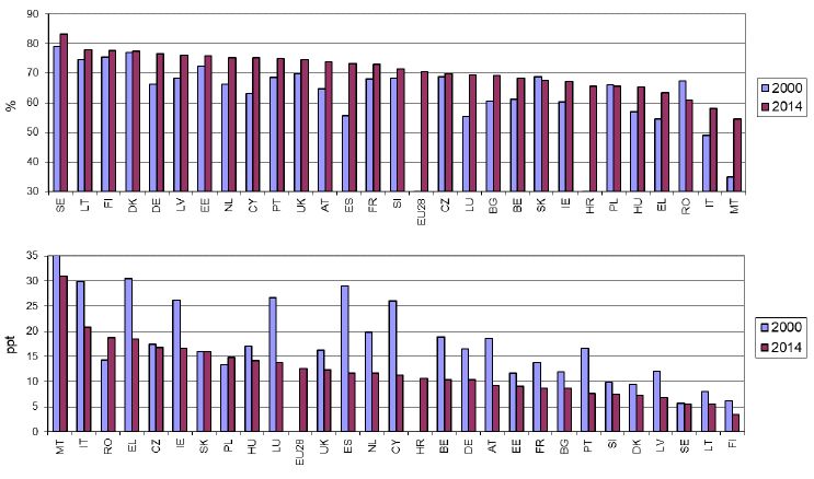
Female participation rates (top panel) and gender participation gaps (bottom panel). Age group: 20–64.

Female employment rates (top panel) and gender employment gaps (bottom panel). Age group: 20–64.
The European Commission (2000) proposed a Community framework strategy on gender equality for the period 2001–2005, which aimed, among other objectives, at strengthening the gender dimension in the European Employment Strategy. Equal employment opportunities and work-family balance are pointed out as priorities. This was followed by the European Pact for Gender Equality and the Roadmap for equality between women and men 2006–2010, updated in the Strategy for equality between women and men 2010–2015 (European Council, 2006; European Commission, 2006, 2011). In these documents, the European Commission proposed concrete actions for addressing a number of issues such as economic independence of women and equality in decision making. The Europe 2020 Strategy, by acknowledging that “policies to promote gender equality will be needed to increase labour force participation thus adding to growth and social cohesion”, sets among its targets for 2020 an overall employment rate of 75% across the population (see European Commission, 2010, p. 17). Furthermore, in the Social Investment Package, the European Commission (2013) reaffirmed the importance of fostering higher participation of women. According to this document, gender gaps in employment rates, as well as other gender disparities in the labour market, need to be reduced or eliminated in order to decrease the risk of social exclusion and poverty for women and to achieve inclusive growth. Access to early childhood education and care needs to be improved to foster both female employment and children’s life opportunities.
In addition to fostering equality, enhancing women’s access to employment can sustain economic growth, especially when considering population ageing and the expected labour supply shortages across the EU. According to the Organisation for Economic Co-operation and Development (OECD) (2008, 2012), narrowing the gap between male and female employment rates has accounted for half of the increase in Europe’s overall employment rate and a quarter of annual economic growth since 1995.
Notwithstanding the attention paid by policy makers, female labour force participation is still much lower than male participation and only slowly catching up in many countries. These differences are to some extent rooted in culture and social norms but they also reflect differences in the economic and demographic structure, as well as institutions and economic incentives. Figure 3 shows raw cross-country correlations between female participation rates and some key demographic and economic variables, at the EU level. Female participation appears to be only loosely related to population ageing, with if anything more participation in countries with an older population, and positively related to fertility rate, education, and the generosity of family policies. The large literature on the determinants of female labour force participation (see for instance Saurel-Cubizolles et al., 1999; Bratti, Del Bono, & Vuri, 2005; Attanasio, Low, & Sanchez-Marcos, 2008; Genre, Gomez-Salvador, & Lamo, 2010; Cipollone & D’Ippoliti, 2011) has investigated these relationships in a multivariate setting, stressing the role of composition effects (for example female participation is higher, on average, in countries with an older population because the share of students is lower and because the share of mothers with young children is also lower) and reverse causation (for example women can better afford having children if they have a job). The complexity of the relationship between demography and labour force participation also points to a crucial role of policies. Thévenon (2011) performs a principal component analysis aimed at identifying the most important characteristics of family policy packages in OECD countries. He finds two main components: one related to support allowing parents to combine work with childcare, and another related to the generosity of leave entitlements in terms of money and duration. Across the range of these two components, he notes that countries adopt one of five broad categories of family policy, of which the ‘Nordic’ family package, based on continuous, strong support for working parents, seems to be the most effective in promoting gender equality and female labour force participation and employment.
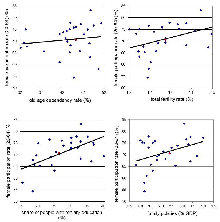

Correlations between the female participation rate and key demographic and economic variables in the EU28 countries. Red dot: EU28 average.
3. Country selection
We present long-term projections for a selection of EU Member States: Sweden (SE), Italy (IT), Spain (ES), Ireland (IE), Hungary (HU) and Greece (EL). Table 1 reports the participation subindex of the Gender Equality Index, computed by the European Institute for Gender Equality (2015) that considers both the gender gap, and the overall level of achievement. Sweden is the best performer, while the other countries included in our focus rank among the most problematic.4
Gender Equality Index: Participation.
| Country | Index | Country | Index |
|---|---|---|---|
| Sweden | 94.7 | France | 75.0 |
| Denmark | 85.3 | Bulgaria | 72.9 |
| Finland | 85.3 | Slovakia | 72.3 |
| Estonia | 83.6 | Romania | 71.8 |
| Latvia | 80.8 | Luxembourg | 71.3 |
| Lithuania | 79.8 | Poland | 71.1 |
| Cyprus | 79.6 | Ireland | 69.8 |
| Portugal | 78.4 | Spain | 69.5 |
| Slovenia | 77.4 | Hungary | 67.5 |
| United Kingdom | 77.4 | Belgium | 66.9 |
| Austria | 77.0 | Croatia | 62.0 |
| Germany | 75.9 | Greece | 59.5 |
| Netherlands | 75.6 | Italy | 57.1 |
| Czech Republic | 75.3 | Malta | 56.2 |
-
Notes: The index ranges from 0 (maximum inequality) to 100 (maximum equality). Countries selected for analysis are in bold.
We investigate the evolution of participation rates in the selected countries by means of a dynamic MSM. In dynamic microsimulations, each individual in a given initial population is evolved through time according to estimated transition probabilities. Different life course events are simulated (for example educational choices, entry in the labour market, household formation and dissolution, fertility, evolution of work careers, retirement, death) with specific MSMs having a focus on different dimensions (for example demography, work, family, etc.) and different subgroups of the population. This has an impact on model specification: for instance, if the focus is on the elderly, issues like retirement choices and disability must be considered in greater detail, while if the focus is on women in fertile years, the former processes can be more vague, while more attention needs to be paid to modelling household composition and its interaction with the working career of mothers. Because of its centrality in life, most MSMs have a labour participation/employment module: see Li and O’Donoghue (2013) for a review. Some are fairly complex models which require years and relatively large teams to build, and that could in theory provide projections on labour force participation with the required focus on the interaction between family choices and career. However, because they have a different primary interest (say, pensions), they do not provide published results on female labour force participation at early stages of the life cycle. Moreover, these large models are all country-specific, and exist only for a limited number of countries.
To the best of our knowledge, the only MSM in the literature with a focus on female labour force participation and its interaction with family life in a European context is Richiardi and Poggi (2014), estimated for Italy, which provides the basis for the model developed here. In addition to improvements in model specification, the new model presented here provides a first example of a multi-country dynamic microsimulation: the structure of the model is the same for all countries considered, and simulations only differ because of country-specific inputs, in terms of representative population samples, estimates and parameters. This feature allows us to obtain results for several countries which are directly comparable in terms of the assumptions and modelling choices made; moreover, it allows running “as if” scenarios, where inputs from one country are tested on a different country (we do so in our companion paper Richardson, Pacelli, & Richiardi, 2016). These benefits are achieved, without excessively complicating the model, by leaving two highly institution-dependent processes in the background: income determination and retirement decisions. While these processes are often the prime object of investigation in dynamic MSMs, our focus on labour force participation and employment, and in particular on participation decisions of women in childbearing years, permits us to treat them at a higher level of abstraction, without compromising the quality of the projections. On the other hand, issues such as household composition and its effects on labour force participation of mothers are considered in detail. Finally, the model can be interpreted as a first step towards a more general model for all EU member states, similarly to what EUROMOD (Sutherland & Figari, 2013) provides for tax-benefit microsimulations.5 In the next section we discuss in more details the pros and cons of the microsimulation approach with respect to what exists in the literature.
4. Methodology
Houriet-Segard and Pasteels (2011) offer a review of the main methods used by governmental institutions around the world to forecast participation rates. Aside from judgmental (or qualitative) methods and simple time extrapolations from historical aggregate data, the most common methodologies are either regression models based on the correlation between participation rates and demographic, economic, and institutional factors, or cohort models.
According to the first approach, a regression model with a set of explanatory variables is fitted on observed (cross-sectional) labour force participation rates. Then, projections for the evolution of participation rates are made on the basis of scenarios for the future evolution of the explanatory variables, including demographic characteristics. According to the cohort model approach, future participation rates are predicted by estimating an age profile of the participation behaviour of the most recent cohorts, appropriately weighted to take into account the (exogenous) demographic evolution. Because cohort models are also based on regressions, in what follows we refer to Houriet-Segard and Pasteels’s regression models as cross-sectional models.
Cohort models are widely used at official agencies like the OECD and the European Commission: for instance, labour force projections in the 2015 Ageing Report are based on a cohort model (European Commission, 2014). In their basic form, cohort models analyse participation rates separately by age group and gender (see for instance Beaudry & Lemieux, 1999; Aaronson, Fallick, Figura, Pingle, & Wascher, 2006; Fallick & Pingle, 2007; Balleer, Gomez-Salvador, & Turunen, 2009). Controls include only aggregate variables, where aggregation is specific to the different gender and age groups: typically, the share of individuals with high/low education, the share of individuals living in different types of households (for example with/without a partner, with/without children), the share of individuals with disabilities, measures of earning potentials such as the (age-specific) gender wage gap, measures of (average) household wealth, measures for business cycle effects, and proxies for the relevant welfare programs, such as the availability of childcare for women in childbearing years, and the fraction of individuals eligible for early retirement in older cohorts. Because each gender-age subgroup provides one unit of observation, the identification of the effects of each determinant can be obtained only by exploiting its variation over time. Time invariant cohort effects are also included. Aggregation over the different gender-age categories is obtained by weighting the participation rates in each subgroup by the population size of that subgroup.
Though cohort models are more sophisticated than cross-sectional models, they basically share common assumptions: (i) both modelling approaches are aggregate, meaning that the units of analysis are groups of individuals, and (ii) the evolution of the explanatory variables is external to the model. The difference lies in the level of aggregation, which in cohort models is taken down to individuals born broadly in the same period (typically, a 5-year or a 10-year window). Participation rates for different cohorts are then aggregated using population weights, while no weighting takes place in cross-sectional models. The results of the two approaches become similar once a full set of demographic characteristics is included among the covariates in cross-sectional models.
This group-level analysis however suffers from what is known as “ecological fallacy” (Robinson, 1950). The ecological fallacy arises when aggregate data are used to infer about the individual level parameters. Many investigators have shown that the aggregate and the individual-level coefficients seldom agree in either magnitude or direction. For instance, it is possible that the individual probability to participate is higher for the majority of individuals in group A, but group B displays a higher aggregate participation rate.6 Also, a characteristic might negatively impact participation rate at the individual level but display a positive association at the aggregate level.7 Avoiding the ecological fallacy is important if one wants to learn about the channels through which the determinants of participation work. This is particularly important when it comes to evaluating or devising policies aimed at fostering participation.
The most sophisticated cohort models get around the ecological fallacy problem by increasing the number of cells (individual characteristics), for instance taking into account differences in skills and family structure. As the number of conditioning variables increases, the approach converges to a microeconometric approach where the estimates are performed at the individual level. Still, the evolution of the weighting variables (for example skills and family structure) for the different groups/individuals is exogenous to the model.8
This is the strategy used, for instance, by Aaronson, Davis, and Hu (2012) and Aaronson, et al. (2014), who estimate the probability of being in the labour force at the individual level, separately by gender and age groups in order to allow the cohort effects and other controls to flexibly vary across age, gender, and education. They control for age, year of birth (i.e. cohort), race, education, the business cycle, plus include additional conditioning variables for specific demographic groups, like the real state minimum wage and the ratio of the average youth hourly wage to average adult hourly wage for the younger age groups, indicators for being married with children and married with a young child for the middle age groups, and gender-specific life expectancies for the older age groups.
As in the microeconometric approaches described above, in the dynamic microsimulation approach (Li & O’Donoghue, 2013) participation is also estimated (and projected) at the individual level. Indeed, the specification of the participation equation in a MSM can be identical to that of an individual-based, microeconometric cohort model. However, the latter are single-equation models, where the outcome of interest (say, the participation rate) is estimated on the basis of individual characteristics — to reiterate, these are just age and gender in the simplest macro-based models, while more individual controls are included in the most sophisticated micro-based models. These individual characteristics define the cells of interest. Aggregate participation rates are recovered as a weighted average of the participation rates in the different cells, using population shares as weights. These weights are then evolved over time based on external scenarios (for example demographic projections). By contrast, in MSMs there are more equations, explaining the evolution, at a micro level, of more variables, including the demographic and economic variables used as controls in the participation equation. Hence, MSMs allow to project participation rates considering the likely evolution of their determinants, at a micro level.9
In dynamic MSMs, each process is estimated at an individual level and feeds back into the other processes in the simulation. For instance, educational choices are simulated and predict, for every individual in the simulation, a level of education at any point in life. This level of education is then taken into account in the simulation of the (individual-specific) probability of entering a consensual union, participating in the labour market, etc. With K processes considered, the general form of a MSM is
where the outcome yk for each process k is simulated for every individual i and time-step t based on the previous individual outcomes of all processes, additional individual characteristics Xi,t and scenario and policy parameters Pt.10
The advantage of the microsimulation approach is threefold. First, aggregation can be performed ex-post on any sub-population of interest (provided it can be identified using the variables included in the model). For instance, we could study the participation rate of mothers with at least one child aged three years old. In contrast, in a cohort model the analysis is restricted to the predefined cells (often, gender and age only). This advantage obviously fades away as the number of characteristics that are allowed to influence the participation rate (the number of cells) increases. Microsimulations are in this respect no different from micro-based cohort models.
Second, and most important, the model provides projections on a possibly large set of outcomes, and not only on one variable. This is valuable even if we are interested in just one outcome y1 (say, labour force participation): the model produces conditional forecasts of y1 given the evolution of other determinants y2, …, yK, plus projections for the likely evolution of those determinants. In contrast, a cohort model provides projections for y1 under the assumption that all the variables which do not define groups remains constant, and conditional on external projections for the evolution of the variables that define groups (the weighting variables).
The third advantage is a consequence of the multi-process nature of dynamic microsimulations and relates to uncertainty assessment. Microsimulations allow an integrated assessment of the uncertainty surrounding the projections, based on the uncertainty of the underlying estimates for all the different processes that compose the model. On the other hand, uncertainty of the projections, even in the most sophisticated cohort models, can only come from the uncertainty surrounding the estimates of the single equation (for example participation). As this is generally not considered, uncertainty assessment in this type of models often boils down to running multiple scenarios about the exogenous evolution of the weights attributed to the different cells, but the choice of these scenarios, and their likelihood, remains outside the scope of the model. Unfortunately, uncertainty analysis is also generally neglected in dynamic microsimulation modelling, so that the advantages of an integrated assessment remain unexploited. An explicit and formal assessment of the uncertainty around our baseline projections is an innovative feature of our analysis. We elaborate on this point in Section 7.
Obviously, in the face of the benefits outlined above, there is a price to pay for the integrated microsimulation approach, in terms of (i) higher model complexity, and (ii) increased data requirements. If the sub-populations of interest are defined only in terms of exogenous variables such as gender and the age structure —considering, at a first approximation, the age structure as exogenous— the extra burden of a MSM might not be worth the costs. On the other hand, if the sub-populations of interest are defined in terms of clearly endogenous variables such as family composition, microsimulations offer a better and more comprehensive theoretical framework.
5. The microsimulation model
The MSM, based on Richiardi and Poggi (2014) and Leombruni and Richiardi (2006), receives as an input a representative sample of the population in each country, drawn from the 2012 wave of EU-SILC11 data —the last available wave at the time the model was implemented— plus the estimated coefficients and tables for the scenario parameters. The microsimulation is composed of four different modules: (i) Demography, (ii) Education, (iii) Household composition, and (iv) Labour market. Each module is in turn composed of different processes, or sub-modules as plotted in Figure 4 (more details on the specification of each module are given in Appendix A).
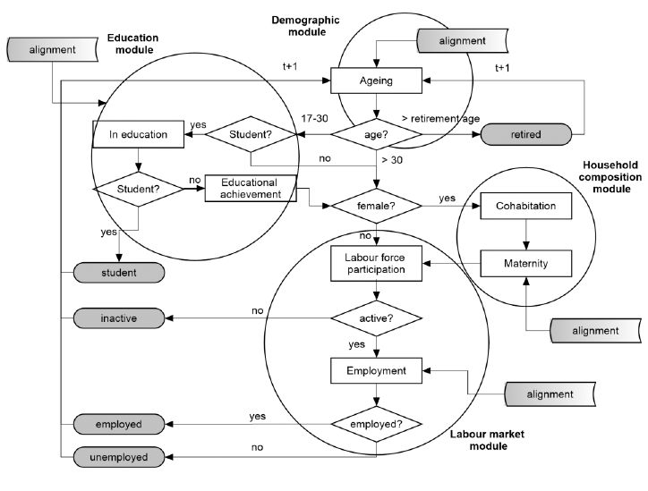

Model structure.
The model simulates the following state variables of the individuals: age, gender, region, educational attainment, labour market status (student, employed, unemployed, retired or other inactive), cohabitation status (for females only) and number and age of children (for females only). Table 2 lists all the equations estimated in the model, identifying outcome variables and determinants (the estimates, together with filtering conditions, are reported in Appendix A). In choosing the specifications for the different equations, we looked at the ‘usual suspects’ identified in the literature (see Del Boca & Wetzels, 2007; and Boeri, Burda, & Kramarz, 2008 for surveys), while taking two considerations into account. First, specifications are kept as lean as possible in order to limit the number of non-significant coefficients, which would increase the variance in the simulated outcomes once the uncertainty of the coefficients is taken into account (more on this in Section 7). Second, specifications are general enough to adapt to the different country characteristics. The equations are estimated on the 2005–2011 waves of the EU-SILC longitudinal panel, the maximum number of waves available at the time.
Causal relations can be highlighted as follows: the education module determines whether the individual continues as a full-time student or if s/he leaves education in t; this depends on age and gender, that is, on demographic characteristics only. If s/he leaves education, the household composition module determines —for women only— whether they move to cohabitation and whether they have a child; this depends on status at t-1, education, age and on having children already. Finally, men and women enter the labour market module where they decide first if they participate and then if they are actually employed, conditional on their family composition, education, and status at t-1. Then they age and go back to the household composition module or to the education module, depending on whether they have left full-time education in the past or not. Everything is conditional on Region of residence.
Inclusion of the lagged dependent variable in most processes is of course problematic: the effects of true persistence, as captured by the lagged status, are estimated with error (typically, overestimated) in presence of unobserved heterogeneity (UH), as discussed in Richiardi and Poggi (2014). Fully accounting for UH is however complicated, especially when the available data have a short longitudinal component, as in the EU-SILC. It is possible to show that including the lagged dependent variable, with high predictive power, and neglecting UH is optimal when one is interested in cross-sectional averages, as in our forecasting exercise —see Richiardi (2012). Clearly, using the MSM for analysing individual trajectories would require more caution in the treatment of UH, and possibly also the inclusion of more lags in the specification of the different processes.
Individuals effectively enter the simulation at age 17, the first age observed in EU-SILC data. The initial population is then evolved forward in time from 2013 to 2050 according to the estimated coefficients and the scenario parameters. Time is discrete, with one period corresponding to one year: correspondingly, all models are discrete choice models (either probit or multinomial probit) with the outcome variable being the probability of occurrence of a given event/transition. In each period, agents first go through the Demographic module, which deals with evolving the population structure by age, gender and area, based on Eurostat official demographic projections. Then, individuals above an individual-specific age threshold retire. Retired individuals remain in the simulation until they die but nothing else happens to them, except the ageing process. As in Richiardi and Poggi (2014), alignment of the population to the official statistics is made by randomly removing individuals from their age-gender cell when the concentration of the cell is higher than in the demographic projections for the specific year, or randomly cloning individuals when the concentration is lower. Students enter the Education module. If they remain in education, nothing else happens to them until the next period. If they exit education, they join the ranks of potentially active individuals. Females enter the Household composition module, where it is determined whether they form or remain in a union and whether they give birth to a child. Then, they join males in the Labour market module, where participation and employment are finally determined.
Determinants of the estimated processes at an individual level.
| Outcome | Determinants |
|---|---|
| Student | age, gender, region |
| Education | age, gender, region |
| Consensual union (female only) | age, student(t−1), education, participation(t−1), cohabitation(t−1), children(t−1), region, retired(t−1) |
| Maternity (female only) | age, student(t−1), education, participation(t−1), cohabitation(t−1), children(t−1), region, fertility rate, public childcare, maternity benefits, part-time rate |
| Participation: women with children aged 0–3 inclusive | age, student(t−1), education, participation(t−1), cohabitation(t−1), region, public childcare, maternity benefits, part-time rate, post-crisis dummy |
| Participation: women with children aged 4–12 inclusive | age, student(t−1), education, participation(t−1), cohabitation(t−1), region, part-time rate, post-crisis dummy |
| Participation: women without children aged 0–12 inclusive | age, student(t−1), education, participation(t−1), cohabitation(t−1), region, post-crisis dummy |
| Participation: men | age, student(t−1), education, participation(t−1), region, post-crisis dummy |
| Employment | age, gender, student(t−1), education, participation(t−1), unemployment rate, region, post-crisis dummy |
-
Notes: Determinants annotated with (t−1) symbolise that the one-period (one year) lag is used.
We now discuss the most important assumptions in the construction of the model, which, as in any model, is based on a number of simplifications.
Education
Individuals never re-enter formal education once they have left it. This is clearly an oversimplifying assumption but is compensated by the fact that education levels are aligned to external projections (see Appendix A.3). This clear temporal distinction between time in education and adult life beyond formal education motivates the assumption that students do not enter the other modules of the simulation (though a flag for individuals who have just left education is present in all equations, see Table 2). Hence, students cannot marry, they cannot have children, and they cannot work, in the model. Testing these specification restrictions in the EU-SILC data is difficult, because EU-SILC data only record whether individuals are in education or not12, and not the number of hours per week spent in education, nor the type of the education course.
Moreover, apprentices are also considered to be in education. Therefore, many individuals show up as “in education” at later stages in life possibly because they are following on-the-job or minor training programs.
Retirement
Given that the primary focus of the microsimulation exercise is not on the elderly, individual behaviour with respect to retirement decisions is kept as simple as possible, while preserving individual heterogeneity. When individuals first enter the simulation, they draw a percentile in the distribution of retirement age. This determines a time-specific individual threshold for retirement (the threshold follows the evolution over time of the average retirement age). In each year, individuals check whether their age is above their (time-specific) threshold: if this is the case, they retire. This approach allows to abstract from the details of the specific pension reforms implemented in each country and is motivated by the observation that the average age of retirement changes shows a high degree of persistence, as depicted in Figure 5 and Figure 6 (the within-country variance remains substantially constant).
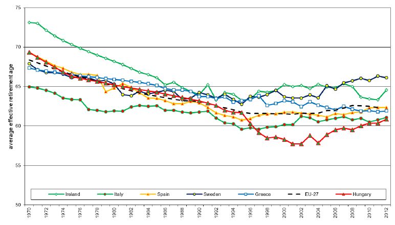

Average effective age of retirement – men.
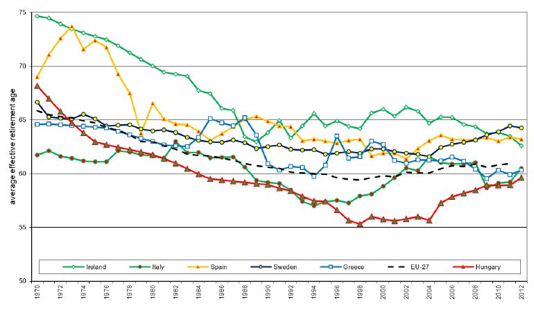

Average effective age of retirement – women.
Maternity
The probability of having a child is estimated around an overall fertility rate coming from the Eurostat demographic projections, and it is aligned ex-post so that, in aggregate, the official projections are met. This means that the total number of new-born children in each year is externally given, and that the microsimulation is used to distribute the births among women in fertile years, given their individual characteristics. The underlying assumption is that the microsimulation is not relied upon to provide demographic projections (it is not constructed to be a “good” demographic model at the aggregate level) but can accurately model heterogeneity in outcomes (it is a “good” demographic model at the micro level, i.e. a “good” model of differential fertility around a given exogenous trend). More details about the alignment algorithm used are given at the end of this section.
Participation and employment
Labour market outcomes are modelled with a double hurdle approach: first we determine participation; then employment, given participation (Blundell, Ham, & Meghir, 1987). The alternative is to have a discrete choice model of hours worked à la Aaberge, Dagsvik, and Strøm (1995) or van Soest (1995), where a set of possible choices are considered based on individual optimisation over leisure and consumption and zero hours are interpreted as non-employment. On the other hand, modelling participation as a separate process allows to distinguish non-employment into unemployment and non-participation.
Given that we do not have monetary variables (that is, wages, other forms of income, savings, and wealth) and we do not explicitly model consumption, there is little advantage of having a “structural” model explaining hours worked.13 Consequently, employment is a dichotomous variable in the model, although the average number of hours worked can be inferred, at an aggregate level, given the predicted employment rates and the assumed evolution of the share of part-timers. This latter variable is a scenario parameter, computed at an aggregate level over the whole working population, and catches not only the structure of labour demand by firms, but also preferences and a general attitude towards family-work life balance. The underlying assumption is that this variable is exogenous: the overall availability of part-time job opportunities in the economy affects the participation rates of female with children, but their participation decisions do not affect (have only a minor effect on) the overall share of part-timers, computed across genders, ages and family structures.
Demand side (business cycle) constraints are taken into consideration by including the overall unemployment rate among the determinants of individual employment.14 This effectively makes the employment module a model of differential employment (analogous to the maternity module), where the overall unemployment rate is a scenario parameter and catches the interaction between supply and demand, which remains outside the scope of the model. The microsimulation then distributes employment among the active population, based on individual characteristics (see Appendix A).
The model further assumes that demand side constraints do not affect participation at the extensive margin (that is the first hurdle). In reality, discouragement can take place and deter individual participation when work opportunities are limited; conversely, a tight labour market can attract new people into the labour force. The justification for not including demand side variables (for example the unemployment rate) into the participation equations is that at the aggregate level this would imply having a model of labour force participation that depends on unemployment, which in itself is defined conditional on being part of the labour force: the unemployment rate is an endogenous variable and including it would deteriorate the quality of the estimates of the other coefficients, and hinder interpretation. Distinguishing between the two hurdles, where the second hurdle is a model of differential employment over the business cycle and the first hurdle is a model of participation that abstracts from business cycles considerations is a good compromise, given that the effects of labour market conditions at the extensive margin are known to be smaller than those at the intensive margin (Attanasio, Levell, Low, & Sánchez-Marcos, 2015).15
For all processes where alignment is performed, we use a resampling procedure (Leombruni & Richiardi, 2006), where individual events are resampled using the estimated probabilities until the target is met. The occurrence of the event (either a 1 or a 0, for example whether an individual is studying or not) are first determined for all individuals in the population. The total is then computed and compared with the target. If the total is above the target (too many occurrences), individuals who were assigned a 1 are asked in random order to redraw their outcome, until the necessary number of switches from 1 to 0 is obtained. If the total is below the target (too few occurrences), a symmetric adjustment takes place, and individuals who were assigned a 0 are asked in random order to redraw their outcome, until the necessary number of switches from 0 to 1 is obtained.
6. Scenario and policy parameters, and baseline specification
The model has the following scenario and policy parameters (Table 3):
Scenario and model parameters.
| Scenario parameters | Differentiated by* | Modules affected |
|---|---|---|
| Initial status at age 17 years | gender and simulation time | 17-year olds |
| Persistence of the effects of the Great Recession | simulation time | Participation |
| Overall unemployment rate | simulation time | Employment |
| Policy parameters | Differentiated by* | Modules affected |
| Average retirement age | gender and simulation time | Retirement |
| Standard deviation of retirement age | gender and simulation time | Retirement |
| Public childcare expenditures | region (NUTS 116) and simulation time | Maternity Participation (females with children aged 3 years or under only) |
| Leave benefits | simulation time | Maternity Participation (females with children aged 3 years or under only) |
| Availability of part-time work | region (NUTS 1) and simulation time | Maternity Participation (females with children only) |
-
*
All parameters (not further distinguished by region) are also differentiated by countries. Simulation time runs from 2013 to 2050.
Initial status at age 17 years
These are the probabilities of being in a specific state at 17 years old, the age at which individuals enter the simulation. States are (i) student, (ii) active (given not a student), (iii) employed (given active). The probabilities of having different education levels, given that an individual has already left education, are also included. The probabilities are distinct for males and females. In all the scenarios considered the probabilities of being in a specific status at age 17 are kept constant throughout the simulation.
Persistence of the effects of the great recession
This is a parameter which can vary between 0 and 1 over simulation time. A value of 1 means that the effects of the crisis on participation rates as detected in the years 2009–2011, on top of the other controls, are still fully deployed; a value of 0 means that they have completely faded away. This parameter assumes a value of 1 in the base year (effects of the crisis as observed in the data) and decreases linearly to 0 up to 2020 (2030 for Greece) in the baseline scenario. It is fixed at 0 afterwards (effects of the crisis completely absorbed).
Overall unemployment rate
This is an alignment parameter that controls the overall unemployment rate in the simulated population. It is allowed to vary over simulation time. The parameter starts from the actual unemployment rate in the last year of observation, and it decreases linearly down to a pre-crisis level in 2020 (2030 for Greece) in the baseline scenario.
Average retirement age
This parameter controls the location of the distribution of retirement age from which individuals draw their actual retirement age, and is primarily controlled by the institutional arrangements. It is distinct by gender and simulation time.
This parameter is increased linearly, separately for men and women, from the values observed in the EU-SILC data to 70 years of age in 2050, for both males and females and in all scenarios. Hence, all countries are assumed to have an average retirement age of 70 in 2050, for both men and women. This should not be considered as a prediction, but rather as a benchmark. Estimates on the likely impact of the pension reforms implemented in recent years, as provided in the 2015 Ageing Report (European Commission, 2015), point to lower average retirement ages. However, these estimates only consider the population in the 50–70 age bracket and are therefore bounded to be lower than 70 by definition. Moreover, they do not take into consideration the need for further reforms, which will likely arise in the forthcoming decades.
An alternative to our simplistic assumption is to extrapolate the trends in average retirement age observed in the data (see Figures 5 and 6). However, the estimates are highly dependent on the initial year which is arbitrarily considered. Moreover, they are also highly heterogeneous, especially for females, reflecting different timing in the implementation of pension reforms in different countries. Extrapolating those trends into the medium/long-term future leads to very implausible predictions. On the other hand, the assumption that all countries will reach an average retirement age of 70 by 2050 implies that countries that are more distant from this target will experience a faster increase. This can be rationalised with higher pressure for reforms, as they might come from super-national authorities (the European Commission, the European Central Bank, the International Monetary Fund, etc.).17
Standard deviation of retirement age
This parameter controls the width of the distribution of retirement age from which individuals draw their actual retirement age and is also primarily controlled by the institutional arrangements. It is in principle allowed to vary across genders and over time. However, since the within-country, within-gender standard deviations of retirement age, as observed in the EU-SILC data, vary only little, they are kept constant throughout the simulation at their average observed values, in all scenarios.
Public childcare expenditures
This policy parameter is distinct by region and simulation time and is measured in USD in purchasing power parity (PPP) per child, as detailed in the OECD Family database. Benefits vary according to the age of the child. Therefore, the total amount of benefits is reconstructed for each family in the simulation based on the presence and age of children. These parameters affect the maternity and female labour force participation modules and are kept constant throughout the simulation: because there are no prices in the model, this is equivalent to assuming that they remain constant also in real terms. In the baseline scenario, their level is that reported in the OECD Family database.
On leave benefits
This policy parameter is distinct by region and is measured in number of weeks of paid parental leave, as detailed in the OECD Family database. It affects the maternity and female labour force participation modules and it is distinct by country. Duration of paid parental leave is kept constant throughout the simulation. As a default (baseline scenario) it is set to the levels reported in the OECD Family database.
Part-time availability
This parameter refers to the overall proportion of part-time work, at a regional level. It is meant to reflect human resource management practices and incentives towards the use of part-time labour, in addition to social norms and family-work balance preferences. It is therefore only partially under the control of decision makers. Part-time rates are also kept constant throughout the simulation, in all scenarios, with a default value equal to that observed in the last year of the data.
7. Assessment of uncertainty
Uncertainty regarding a model’s projections can arise from a variety of reasons (Bilcke, Beutels, Brisson, & Jit, 2011; Creedy, Kalb, & Kew, 2007). In particular, sources of uncertainty are generally distinguished in (i) input data, for instance due to sampling errors in the initial population, (ii) model structure, that is the validity of the general modelling approach used (also called “methodological uncertainty”), (iii) model specification, which concerns the choice of the covariates and the functional forms used, and in particular the crucial assumption that any regularity observed in the data will not break up in the future, (iv) model parameters, pointing to the imprecision of the estimates and/or externally provided parameters, and finally (v) Monte Carlo variation of the model output, which originates from the fact that the simulated aggregate quantities are also imprecise estimates of the theoretical aggregate quantities that the model implicitly defines. None of the above sources of uncertainty is generally considered in microsimulation studies, although this is recognised and criticised (see for instance Goedemé, Van den Bosch, Salanauskaite, & Verbist, 2013). However, “[t]he calculation of confidence intervals around model results that account for all sources of error remains a major challenge” (Mitton, Sutherland, & Weeks, 2000, p. 4).18
In our case, source (i) should be limited, due to the use of the sampling weights provided in the EU-SILC data. Sources (ii)–(iii) are left unexplored, and we make the common assumption that the model is well specified. Measures of fit for each estimated equation are reported in Appendix A, and they are generally appropriate. Monte Carlo variation of the model outcome (source v) can be brought down to negligible by appropriately scaling up the simulated population size.19 The remaining source of uncertainty that needs to be addressed is therefore parameter uncertainty, stemming from sampling errors in estimation (source iv). There are two approaches that can be used to deal with this uncertainty (Creedy et al., 2007). The first is what we might label “brute force” and prescribes to bootstrap the coefficients of the estimated equations from a multivariate normal distribution (in the case of probit or multinomial probit regressions) with mean equal to the point estimate, and variance-covariance matrix equal to the estimated variance-covariance. Bootstrapping needs to be performed only once, at the beginning of the simulation: the entire simulation is then performed with the bootstrapped values of the coefficients. The second approach provides an approximation by assuming from the onset a normal distribution for the resulting confidence intervals, requiring many fewer draws from the parameter distribution. We follow the first approach and draw 1,000 sets of parameter values from their estimated multivariate distribution, for each country in the baseline scenario. Then, for every simulation time, we provide confidence intervals based on a kernel density estimation of the resulting distribution. The results, together with some additional remarks on the uncontrolled sources of uncertainty and the scope of the microsimulation exercise, will be presented in Section 8.3. Here, we only stress once again that the objective of dynamic microsimulation modelling is not forecasting per se, but rather the identification of the forces that are at work at the individual level, and the analysis of how these forces interact in shaping the particular societal outcome of interest. The projections should therefore be considered ceteris paribus exercises with respect to all the dynamics that are not explicitly modelled, and for which an assessment of the uncertainty must rely on external knowledge.
8. Results
8.1 Overall trends
In 2013, only Sweden had an overall employment rate above the Europe 2020 target of 75%. In our baseline scenario, employment rates are predicted to increase in all countries in the simulation period, due to (i) an increase in participation rates, (ii) a gradual recovery from the historically high unemployment rates observed at the beginning of the period, caused by the Great Recession.
Figure 7 depicts the projected employment rates for the population aged 20 to 64 years. By 2020, no other country will have reached the target, though Ireland will be close. According to the projections, the 75% target will be approached only at the end of the simulation period, by 2050, in all countries with the exception of Hungary, which appears to converge towards an employment rate around 71%.
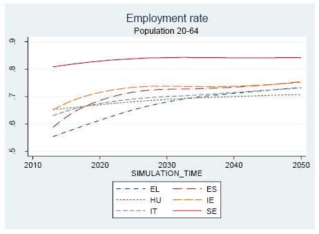
Projected employment rates (20–64 years old), and target line at 75%.
To gain an insight into these projections, Figure 8 reports the simulated participation rates (also called “activity” rates here) in four sub-populations of interests: (a) males aged 20–64 years, (b) females aged 20–64 years, (c) females aged 20–44 years (with or without children), and (d) females aged 20–44 years with children (between 0 and 12 years old).
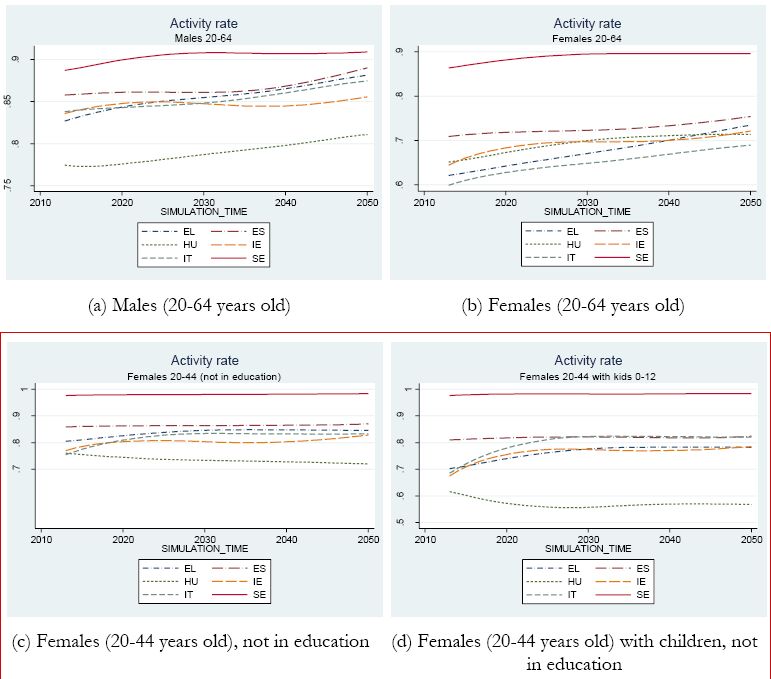

Projected labour force participation rates.
There is a general trend of increasing participation rates towards the very high Swedish levels, which accelerates in the 20–64 years old population (panels a-b) after 2030 when older cohorts are finally replaced by younger cohorts with higher participation rates (panels c-d). The only exception to this general pattern is Hungary, where participation rates of mothers are particularly low and, given the recent trends as observed in the EU-SILC data, are not projected to increase.
This evolution of the labour force is reflected in the projections for employment rates, shown in Figure 9, where the sharp increase up to 2020 (2030 in Greece) is due to the hypothesis of a complete recovery from the Great Recession by that year.

Projected employment rates.
8.2 Comparison with the 2015 Ageing Report
These projections, obtained with the microsimulation model (MSM), can be contrasted with those of the 2015 Ageing Report (European Commission, 2015) derived from a cohort simulation model (CSM, see above). For a proper comparison, it should be taken into account that the forecasting horizon and the population at risk in the two models do not match perfectly. First, the Ageing Report offers projections for 2060, while we go as far as 2050: ceteris paribus, given the upward trends in participation, we would then expect higher figures for the Ageing Report.20 Second, the Ageing Report focuses on the 15–64 population, while we need to restrict to the 18–64 population, given that our estimates are based on EU-SILC data21: ceteris paribus, given the low participation rates of individuals aged 15–17, this censoring should drive our figures up. The net effect of these two forces is a priori unknown.
Table 4 compares the participation rates predicted by the two models. When considering the larger age group, we find higher participation rates for Ireland and Italy (respectively 75% vs. 68%, and 75% vs. 65%), while in the 55–64 age group we project a lower rate for Spain (77% vs. 86%), and a higher rate for Ireland (76% vs. 65%) and Sweden (95% vs. 79%).
Comparison of microsimulation model (MSM) outcomes with the projections of the cohort simulation model (CSM) of the 2015 Ageing Report (European Commission, 2015). Labour force participation (male and female population).
| Outcome | Participation rate (%) | Participation rate (%) | ||||
|---|---|---|---|---|---|---|
| Model | Eurostat | CSM | MSM | Eurostat | CSM | MSM |
| Age group | 15–64 | 15–64 | 18–64 | 55–64 | 55–64 | 55–64 |
| Time | 2013 | 2060 | 2050 | 2013 | 2060 | 2050 |
| Greece (EL) | 67.7 | 75.4 | 77.3 | 42.4 | 78.0 | 76.8 |
| Spain (ES) | 74.2 | 78.9 | 79.3 | 54.2 | 82.5 | 76.9 |
| Hungary (HU) | 64.7 | 73.0 | 72.8 | 41.8 | 77.5 | 75.1 |
| Ireland (IE) | 69.7 | 68.2 | 75.2 | 57.3 | 64.6 | 77.5 |
| Italy (IT) | 63.4 | 65.2 | 75.2 | 45.4 | 69.0 | 70.9 |
| Sweden (SE) | 81.3 | 82.3 | 86.3 | 77.7 | 78.9 | 95.1 |
The reader should evaluate the different projections on the basis of the assumptions of the two models. However, focusing on the larger age group, we point out that the CSM predicts a decrease in the participation rate in Ireland from the current level of about 70%, and only a very modest increase (from 63% to 65%) in Italy. This looks at least counter-intuitive.
Table 5 compares the outcomes of the two models with respect to employment and unemployment rates, finding the same qualitative differences as discussed with respect to the participation rates.22
In particular, overall employment rate is predicted to be lower in Ireland and Italy by CSM; the employment rate of the elderly is predicted to be lower in Ireland and Sweden, higher in Spain, by CSM; the unemployment rate is more similar but for Ireland (higher) and Sweden (lower).
Comparison of microsimulation model (MSM) outcomes with the projections of the cohort simulation model (CSM) of the 2015 Ageing Report (European Commission, 2015). Employment and unemployment (male and female population).
| Outcome | Employment rate (%) | Employment rate (%) | Unemployment rate (%) | ||||||
|---|---|---|---|---|---|---|---|---|---|
| Model | Eurostat | CSM | MSM | Eurostat | CSM | MSM | Eurostat | CSM | MSM |
| Age group | 15–64 | 15–64 | 18–64 | 55–64 | 55–64 | 55–64 | 15–64 | 15–64 | 18–64 |
| Time | 2013 | 2060 | 2050 | 2013 | 2060 | 2050 | 2013 | 2060 | 2050 |
| Greece (EL) | 48.7 | 69.8 | 69.6 | 35.5 | 74.6 | 73.8 | 28.0 | 7.5 | 9.9 |
| Spain (ES) | 54.5 | 73.0 | 72.3 | 43.4 | 77.9 | 72.9 | 26.5 | 7.5 | 8.8 |
| Hungary (HU) | 58.0 | 67.5 | 67.2 | 38.6 | 73.6 | 71.5 | 10.3 | 7.5 | 7.6 |
| Ireland (IE) | 60.4 | 63.5 | 71.6 | 51.2 | 61.3 | 76.5 | 13.3 | 6.8 | 4.9 |
| Italy (IT) | 55.5 | 60.3 | 69.7 | 42.8 | 66.7 | 69.5 | 12.4 | 7.5 | 7.3 |
| Sweden (SE) | 74.6 | 77.4 | 80.0 | 73.7 | 76.0 | 92.1 | 8.2 | 5.9 | 7.4 |
Participation rates and participation gaps with respect to Sweden, female population aged 20–64 years, baseline scenario.
| Females (20–64 years old) | |||||
|---|---|---|---|---|---|
| Year | 2013 | 2020 | 2030 | 2040 | 2050 |
| Participation rates (%) | |||||
| Sweden | 86.4 | 88.3 | 89.6 | 89.4 | 89.7 |
| Spain | 70.9 | 72.3 | 71.8 | 73.3 | 75.5 |
| Hungary | 65.1 | 66.8 | 70.2 | 71.3 | 71.3 |
| Ireland | 62.8 | 69.5 | 69.6 | 69.6 | 72 |
| Greece | 62.4 | 64.1 | 67.1 | 70 | 73 |
| Italy | 59.0 | 63.3 | 64.7 | 67 | 68.8 |
| Participation gap w.r.t. Sweden (%) | |||||
| Spain | 15.5 | 16.0 | 17.8 | 16.1 | 14.2 |
| Hungary | 21.3 | 21.5 | 19.4 | 18.1 | 18.4 |
| Ireland | 23.6 | 18.8 | 20.0 | 19.8 | 17.7 |
| Greece | 24.0 | 24.2 | 22.5 | 19.4 | 16.7 |
| Italy | 27.4 | 25.0 | 24.9 | 22.4 | 20.9 |
More disaggregated results for each country are discussed below.
8.3 Uncertainty analysis
As for what concerns the assessment of the uncertainty around the estimates, this is not available for the CSM. On the other hand, Figure 9 reports a distributional analysis of the model outcome for the MSM, according to the methodology discussed in Section 7. Shades of grey are proportional to the estimated densities, while the 90% confidence band is also super-imposed. Overall, the uncertainty coming from sampling errors in estimation is small, except for Greece and Ireland (about 10 ppt in the final year of the simulation). This should not however boost our confidence in the model results too much, as the assumption that no general equilibrium feedbacks will intervene to modify the regularities found in the estimation data becomes more and more unwarranted as we extend our out-of-sample projections into the future. Moreover, projections also abstract from unforeseen shocks, both at a micro-level (such as an unexpected surge in migration flows) and at a macro-level (such as the potential consequences of a breakdown of the Eurozone, or the shock waves caused by a hypothetical exit of a big member state, like the United Kingdom, from the EU), which also increase (in expectation) the uncertainty surrounding the model results as the forecasting horizon increases.
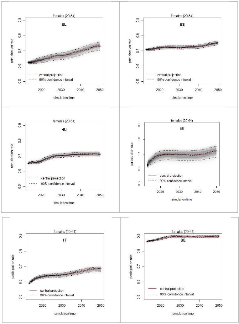
Uncertainty analysis.
8.4 Country projections
In this subsection we discuss country results in more detail. We begin with Sweden, our benchmark country; then consider the other countries in decreasing order of population size: Italy, Spain, Greece, Hungary and Ireland. We focus on the female population, and present projections for both the main determinants (education and family composition) and outcomes (labour market status). All tables for the country results are reported in Appendix B.
8.4.1 Sweden
We first look at the evolution of the main characteristics of the female population in the 20–64 years age range. These are reported in Table B.1.1. Starting from the current high levels, the share of women with high education is expected to rise further, while the current gender participation gap (see Figure 1) is expected to close. The dynamics for employment closely follow those of participation, given the assumptions of the model (hence they are not reported in the table).
When we focus on the 20–44 female population (Table B.1.2), no big changes are expected, which strengthen the case for Sweden as a benchmark country. Participation rates among the 20–44 years female population remain high and approximately similar also when disaggregating by region, education and family composition (Table B.1.3). In particular, there are few differences between the region with the highest participation rate (SE1, in 2013) and the region with the lowest rate (SE2, in 2013). Having children in Sweden does not place women at a disadvantage, as regards to participation (and employment). Also, only small differences are found between women with high education, and women with low education. These results reflect the exceptional approach of the Nordic countries regarding family support combined with diversity efforts. It is common and viewed positively when both parents care for their children and, accordingly, the government as well as employers have institutionalised numerous work-life balance programs combined with incentives for young families (European Commission, 2013a). Part-time arrangements are well established in the Swedish business community as they go hand in hand with the extensive public benefits for young parents. Sweden was the first country to grant men and women equal access to paid parental leave in 1974. Parents are entitled to a total of 480 days paid leave per child, with both mothers and fathers entitled and encouraged to share the leave. This is paid at 80% of the salary (up to a ceiling) for 65 weeks, and at a flat rate for the remainder. However, because few men took parental leave, a non-transferable “daddy’s month” was introduced in 1995, extended to two months in 2002 (Addati, Cassirer, & Gilchrist, 2014). There are additional programs and incentives to promote a high quality of family life. Childcare access is universal and almost free of charge (Garcia-Moran, 2010). The result is that 51% of children under the age of three and 95% of children between three and school age were enrolled in formal childcare (European Commission, 2013b).
Finally, we look at females in the 55–64 years age group (Table B.1.4). The high participation and employment rates of the elderly are the result of strong incentives to remain in the labour market at later ages, in terms of income tax credits and reduced employer contributions for workers aged 65 and over (Eurofound, 2012). Here, again, no significant regional differences are found. However, in this age group education makes a difference, with approximately a 15 ppt gap in participation rates between high and low educated females. This gap is expected to shrink to about 10 ppt by 2050.
8.4.2 Italy
Low female participation has always been a feature of the Italian labour market (Del Boca et al., 2005). In particular, participation rates of mothers with young children are still very low (Del Boca, 2003): more than a quarter of women leave the labour market after a birth (Bratti et al. 2005; Casadio, Lo Conte, & Neri, 2008). Italian women often do not participate in the labour market as their role in the family limits their possibilities to pursue a career (European Commission, 2013c). In fact, Italian women face a general cultural attitude against female labour force participation, a lack of part-time opportunities, a disproportionate share of the burden with respect to housework and child bearing within the family and an inadequate public childcare system. Concerning the enrolment in full-time childcare facilities (30 hours or more per week), Italy ranks above the EU average for children from zero to three years of age (17% vs. 15%), as well as for children from three years to school age (75% vs. 47%, see European Commission, 2013d). However, the high cost of childcare services remains a problem. Moreover, the hours of childcare offered are typically incompatible with full-time jobs. As for what concerns children of school age, things do not improve much as school days often end in the mid-afternoon, much earlier than the end of fulltime workdays (Del Boca, 2002; Del Boca & Vuri, 2007). This helps explain why the overall labour market participation of women in Italy still remains one of the lowest in Europe, with only 57.2% of active women in the 20–64 years age group in 2013, despite an increase in recent years. On the other hand, male participation is in line with the EU average (83% in 2013). This translates into a large gender gap (26 ppt).
In our baseline scenario, however, family policies and part-time opportunities are kept constant, so they do not explain the predicted increase in female participation, especially for younger cohorts, and the slight decrease in the gender gap, as shown in Figure 6. Our explanation points to another determinant of the low female participation rate in Italy, and how it interacts with family composition: low education. Italy has the lowest level of educational attainment among EU countries, and this affects female more than male labour force participation: the proportion of the population aged 30 to 34 with tertiary education in 2013 was 19% among males, and 29% among females, against an EU average of 34% and 42% respectively, and way behind the Europe 2020 target of 40% (the national target is 26%). This educational gap is even bigger when considering the whole population, due to the weight of older cohorts with lower levels of education (Table B.2.1). On aggregate, educational attainments in the model follow the external forecast: they are projected to grow but will remain low with respect to the EU average. However, the model predicts a change in the behaviour of young women, partly as a consequence of delayed marriage (Table B.2.2) which will force single women to be more active. In particular, the participation rate among young women with low education, both with and without children, is expected to increase significantly, leading to an overall increase in the participation rate in the 20–44 age group (Table B.2.3). This however will not be sufficient to outweigh the behaviour of older cohorts, leading to an overall female participation rate in Italy that is expected to remain the lowest in the countries under investigation (Figure 6, panel b). Regional differences are also expected to remain large, notwithstanding a reduction in the gap between the highest and the lowest participation regions for younger cohorts (from 30 to 20 ppt, see Table B.2.3). Regional and educational differences in female participation rates are on the other hand projected to remain almost unchanged in the older cohorts (55–64 age group, Table B.2.4).
8.4.3 Spain
For the last two decades, Spain has witnessed an increase in access of women to the labour market, achieving participation rates above the EU average. A substantial part of this increase concerns the rise in the labour force participation rate of mothers (Borra, 2010), and can be explained by an overall good level of family support, though this comes mainly in the form of child related benefits, while public childcare infrastructures for the age group from zero to three years old are still inadequate.23 This results in the common use of private childcare: over 20% of children under three and 50% of children between three and school age are enrolled full time (30 hours or more per week) in formal childcare (European Commission, 2012a). Moreover, Spain provides for 16 weeks of fully paid maternity leave around childbirth, conditional on previous work experience; there are also legal entitlements to paternity leave (four weeks, fully paid) which often help mothers to get back to work (Borra, 2010; Ibáñez, 2010).
However, women still do not participate in the labour market to the same degree as men and the female participation rate is still low compared to that of northern European countries. In 2013, around 71% of Spanish women aged 20 to 64 were active, as opposed to 86% of Spanish men, resulting in a gender gap of 15 ppt. Participation rates are predicted to remain fairly constant in Spain until 2030, and then slightly increase (about three ppt both for males and females) between 2030 and 2050 (see Figure 7, panels a-b, and Table B.3.1). Except for a decrease in the share of women living inside a union, which is common to all countries except Sweden and Ireland, the characteristics and behaviours of the Spanish population will not change much (see Tables B.3.1-B.3.3 for the female population; similar dynamics also hold for the male population). Consequently, the predicted increase in participation rates is entirely explained by composition effects, and in particular by demographic change. In fact, participation rates of older age groups show a larger increase (see Table B.3.4 for females; a similar pattern is found for males), as the older cohorts exit working age and are replaced by new cohorts.
8.4.4 Greece
Projections are obviously impervious for Greece, a country battered by a harsh recession and unprecedented macroeconomic challenges. Still, it is interesting to analyse the long-run implications of the dynamics detected in the data, referring mostly to a period prior to the recession, which provide an assessment of the potential of the Greek economy if the external macroeconomic constraints would be relaxed.
Since the 1980s, the combination of more employment opportunities in the tertiary sector, more educational opportunities for women and the extension and improvement of public child and elderly care services have propelled the steady increase in female labour force participation in Greece (European Commission, 2012b; Bugra & Özkan, 2012). In particular during the 1990s, pregnancy, maternity and parental leave were guaranteed by law, childcare and elderly care facilities were expanded, and benefits and tax exemptions for families with children were implemented (Kanellopoulos & Mavromaras, 2002). Thus, to achieve their labour market objectives, Greek women acquired higher levels of formal education, delayed marriage and reduced childbearing, though to this day, full-time work is still often not possible without the help of other family members (Kanellopoulos & Mavromaras, 2002).24 Table B.4.2 shows that the trend towards delayed marriage and reduction in the number of children is likely to continue in the future.
The unleashing of the dynamics analysed above has the potential to increase the participation rates of all segments of the Greek female population further, and in particular of mothers in childbearing age (Table B.4.3), though the projections have a higher degree of uncertainty than in the other countries analysed thus far (see Figure 8). However, regional and educational differences are expected to persist over time (Table B.4.3), while educational differences in participation rates for the elderly female population are likely to widen, due to a sharp increase in the attachment to the labour force of more educated women (Table B.4.4). This has to be evaluated taking into consideration that female labour force participation among elderly women in Greece is one of the lowest rates in Europe, with family reasons being cited as the most likely factor associated with inactivity. In fact, previous breaks in working life resulting in fewer career options later on, combined with lack of care facilities can push senior females out of the labour market to provide care for grandchildren or older family members.
8.4.5 Hungary
Hungarian women are more educated than men, on average, and do not face discriminatory legal restrictions when it comes to owning property, starting businesses or participating in the labour force (Gonzalez et al., 2015). However, women are significantly behind when it comes to employment and this situation is projected to persist over time (see Figure 7). One of the reasons is the strong negative effect of childbearing: in particular, women with children and a low education have an extremely low attachment to the labour market (less than 45% for women with children aged 12 or under, see Table B.5.3).
These low levels of participation originate from very strong disincentives to work for mothers with very small children (aged three or under). In this group, the participation rate was only 13% in 2013, and was also very low among the highly educated (20% in 2013). In Hungary, work disincentives predominantly arise from the design of extended paid parental leave, in a context of a shortage of affordable childcare (Jenker, 2015). Parents can take up to three years of leave, and the overwhelming share of caregivers are women (Korintus & Gábos 2014). Benefits are entitled to mothers of young children staying at home: maternity leave and the insurance-based childcare benefit can only be taken until the child’s first birthday; and a mother receiving these benefits cannot work. Extended leave periods (beyond 24 months) tend to negatively impact female participation by weakening mothers’ attachment to the labour market and putting them at a disadvantage from a prospective employer’s point of view (European Commission, 2014b). This is particularly true for women with a low education, who tend to remain out of the labour force even when their children grow up. Finally, Hungary also has a significantly lower part-time rate for women than the EU average: women in Hungary tend to work full-time or not at all (European Commission, 2012c).
As in Spain, but at a lower level of participation, activity rates by education and family composition are projected to remain fairly constant during all the simulation period (Tables B.5.2 and B.5.3). Most of the changes in the aggregate participation rates are therefore due to composition effects, arising from demographic change and a strong projected increase in the share of single women, due either to delayed marriage, widowhood or split (Tables B.5.1 and B.5.2). This is reflected in a projected increase in the participation rate of elderly women, as the older cohorts are replaced by new generations (Table B.5.4).
8.4.6 Ireland
Between 1998 and 2007 the female participation rate in Ireland increased sharply as result of strong economic growth, rapid labour market expansion and significant changes in a number of key policy areas (for example, extensions to maternity leave, the introduction of parental leave, individualisation of the tax system and the establishment of a national minimum wage). During this period, the gap between male and female employment rates has been closing bit by bit (Russell, McGinnity, Callan, & Keane, 2009). In the face of these changes, the 2008 recession led to a sharp turnaround of the Irish economy. In just a few short years, Ireland passed from having the highest GDP and employment growth in Europe to being among the countries with the highest unemployment, emigration and debt levels (Barry & Conroy, 2013). Indeed, Irish employment rates among both men and women were above the EU average before the recession (surpassing the EU Lisbon employment targets) but they had fallen significantly below the EU average by 2012 (Barry & Conroy, 2013).
Employment rates are expected to increase by approximately 10 ppt between 2013 and 2050, with most of the increase taking place before 2025 (Figure 6). The dynamics of employment (Figure 8) are stronger than those of participation (Figure 7), as they incorporate a complete recovery by 2020 from the high unemployment rate observed at the beginning of the simulation period. However, the Europe 2020 target of a 75% employment rate in the 20 to 64 age group is likely to be approached only at the end of the period (the uncertainty around the estimates is however bigger for Ireland than any other country except Greece, see Figure 8).
In Ireland, women in the family are expected to deliver care and support across a range of social needs such as caring for children and people who are long-term frail or with disabilities. Part time opportunities to reconcile work and family duties are higher compared to the EU average (European Commission, 2013c). However, female participation is constrained by many barriers such as the absence of decent and affordable childcare, afterschool care and elderly care, discrimination in the workplace, a poor provision of maternity leave, absence of parental leave and an expansion of low-paid atypical employment in the service sector (Barry & Conroy, 2013). Only 11% of children between zero and three years of age receive 30 or more hours of childcare per week (the EU average in this age group is 15%), while 82% of children between three years old and school age are enrolled in formal childcare (European Commission, 2013d).
Education is a key factor influencing female labour force participation in Ireland, especially in childbearing age (European Commission, 2013d). Higher educated women have greater participation rates in general, but the gap is larger for women with children (over 30 ppt, see Table B.6.3). This gap is expected to reduce, but only slightly (to approximately 25 ppt) during the forecasting period.
Similarly, the gap in participation rates between high and low educated females in the 55 to 64 years age group (Table B.6.4) is very large (almost 50 ppt) and is expected to shrink (by approximately 10 ppt), though it will still remain high (about the same size of the gap in Italy, Spain and Hungary).
9. Summary and conclusions
In this paper, we have presented a dynamic MSM of educational choices, household formation and labour market outcomes (participation and employment), that we have then applied to derive medium- and long-term projections for a selection of EU member states characterised by low labour force participation rates (Italy, Spain, Greece, Hungary and Ireland, in decreasing order of population), with a high-participation benchmark represented by Sweden.
The microsimulation approach has several advantages over simpler and more common methodologies. Most importantly, it produces forecasts not only on the outcomes of interest (participation and employment in our case) but also on their determinants (for example educational attainments, household composition). Related to this, it allows a more comprehensive assessment of the uncertainty around the projections, given that the evolution of the determinants is endogenous to the model rather than being exogenously provided, though this is very rarely done in microsimulation modelling. Finally, having the individual rather than a group of individuals as the basic unit of analysis allows to study the dynamics of any sub-population of interest (provided it can be identified using the variables included in the model), rather than being constrained by an ex ante choice of a (generally limited) set of characteristics.
From a methodological perspective, two features of our study are noteworthy. First, the model is, to the best of our knowledge, the first dynamic microsimulation exercised to be applied simultaneously to a number of different countries, providing homogenous results which can be directly compared. Second, we offer a thorough discussion of the uncertainty surrounding our projections, quantifying both the sample size required to keep Monte Carlo variation sufficiently low, and the effects of sampling errors in the estimation of the underlying equations.
Results of the baseline scenario identify a general trend of increasing participation rates towards the very high Swedish levels, which accelerates in the 20–64 population after 2030 when older cohorts are finally replaced by younger cohorts with higher participation rates. The only exception to this general pattern is Hungary, where participation rates of mothers are particularly low and, given the recent trends as observed in the EU-SILC data, are not projected to increase. However, Sweden will not be joined by any other country in our sample in meeting the Europe 2020 target of a 75% overall employment rate by 2020, though Ireland will be close. According to the projections, the 75% target will be approached only at the end of the simulation period, by 2050, in all countries with the exception of Hungary, whose employment rate is projected to increase only to slightly more than 70%.
These projections are not too dissimilar from other forecasting exercises in the literature. In particular, we reach the same conclusions of the 2015 Ageing Report (European Commission, 2015), in the aggregate, with respect to Greece, Spain and Hungary, while we are less pessimistic than the 2015 Ageing Report with regards to Italy and Ireland. However, our microsimulation approach permits a finer disaggregation of the results, which turns out to be crucial in understanding the dynamic causal mechanisms at work, as explored further in our companion paper (Richardson et al., 2016).
Footnotes
1.
Life expectancy is up approximately from 70 to 80 years, mean years of education is up approximately from 6 to 11, and retirement age is down approximately from 68 to 63. Figures are approximate as historical data are not available for a number of EU28 Member States. We computed approximate averages based on the available data. Source: Eurostat, OECD, United Nations.
2.
Eurostat projections.
3.
The rationale for country selection is described in more detail in Section 3.
4.
The low ranking of Belgium might look surprising at first. Belgium has a relatively moderate gender gap (11.1 ppt in 2014, computed on the whole population, against an EU28 average of 13.1 ppt) but is penalised by its overall low participation rates (53.5%, against an EU28 average of 64.9%). Source: OECD.
5.
Tax-benefit microsimulations are also called static microsimulations because they provide only estimates of the “day-after” effects of given policy changes (typically incorporating labour supply behavioural responses), for a fixed population. In contrast, dynamic microsimulations take into account demographic change, and focus on long-run dynamics.
6.
Suppose there are 1000 individuals in each group. 800 individuals in group A have a probability to participate of 50%, while the remaining 200 individuals have a probability to participate of 0. In group B, 800 individuals have a probability of 40%, and 200 individuals have a probability of 100%. Individuals in group A are more likely to participate than individuals in group B; however, the participation rate is higher in group B (52% versus 40%).
7.
As an example, individual wealth might have a negative impact on participation, but aggregate wealth could affect participation even after controlling for individual wealth. This could happen for instance if people are trying to “keep up with the Joneses”, reacting to relative wealth. If the distribution of wealth is skewed enough, a positive association between wealth and the participation rate would be detected, at the aggregate level.
8.
In these more sophisticated models, the estimation of behavioural responses, where the number of hours worked depends for instance on the tax and benefit system as in Dolls, Doorley, Schneider, and Sommer. (2013), allows to evaluate the effects of proposed policy changes. However, the results still depend on the assumption that the evolution of the weighting variables (for example skills and family structure) is not affected by the policy changes.
9.
For a more in-depth comparison of the different projection approaches, see Comas-Herrera, Wittenberg, and Pickard (2004).
10.
Some (or all) processes may be cast in continuous time (i.e. be specified in terms of duration models). This does not impinge on the general representation of Equation 1, as all continuous-time processes map unambiguously into a discrete-time representation (but not vice versa).
11.
2011 for Ireland.
12.
variable PE010.
13.
These are common in static tax-benefit microsimulation models, which focus on the behavioural responses of labour supply to a change in the gross-net income conversion (that is, the tax and benefit system) at the extensive (that is, participation) and intensive (that is, hours worked) margins.
14.
This is a reduced-form approach to modelling demand-supply interaction. For a more structural approach, which requires modelling wages and is outside the scope of the present model, see Peichl and Siegloch (2013), or Lichter, Siegloch, and Peichl (2014).
15.
We acknowledge that the demand side of the labour market is crucial in the evolution of participation and employment rates, and that here we impose a shortcut to deal with it. A full-blown module of labour demand is beyond the scope of the present work but is high on our agenda for future developments of the model.
16.
first-level ‘Nomenclature of Territorial Units for Statistics’, a geocode standard for referencing the administrative divisions of countries for statistical purposes, developed by the EU.
17.
Indeed, the expected effects of the reforms already implemented are stronger in countries with current lower average retirement age, such as Greece and Hungary (see Figure 4).
18.
An even greater lack of attention to the issue is found in cohort models — see for instance the projections contained in the 2015 Ageing Report (European Commission, 2015).
19.
In all simulation runs we chose an initial population of 100,000 individuals (coming from the last available wave of EU-SILC data, appropriately over-sampled), which, given the distribution of the characteristics in the subgroups of interests, guarantees that the uncertainty stemming from Monte Carlo variation in the simulated data is tiny (generally a fraction of a percentage point). To see this, assume that the probability of the event (participation) for an individual with characteristics X is p. As predicted by the Central Limit Theorem, the simulated probability
This is the minimum population size that allows the confidence interval to be as tight as required. Suppose we set ME to 0.005 (a confidence interval of 1 percentage point) and we require a 95% confidence interval, with
20.
Pushing our estimates 10 years further, till 2060, would make our forecasts less reliable, as discussed in the text. Given that the focus of the paper is not the comparison with the Ageing Report, but it is more methodological, making the estimates less reliable would hamper the main goal of the paper.
21.
EU-SILC is limited to individuals aged 17 years and over. Individuals enter the simulation at age 17 years, but then are immediately aged. Given that the statistics are collected at the end of each simulation period, we get information only on individuals aged 18 years and over.
22.
The unemployment rate is a scenario parameter in the microsimulation model. Note that the projections in column 3 refer to the 18–64 population and are therefore lower than those depicted in Figures 5a and b that refer, as the Europe 2020 target, to the 20–64 population.
23.
As a consequence of the economic crisis, government–funded support for families has become more restrictive in recent years.
24.
Only 5.0% of all children younger than three years receive childcare for more than 30 hours a week, compared to a European average of 14%, and only 22% of Greek children between three years old and school age attend childcare for 30 hours or more, compared to a European average of 45% (European Commission, 2012b).
Appendix
A The microsimulation model
A.1 Model structure
The forecasting model for the six case studies is a dynamic microsimulation (Li & O’Donoghue, 2013), based on the models of Richiardi and Poggi (2014) and Leombruni and Richiardi (2006). It is implemented in the Java programming language using the JAS-mine microsimulation platform (Richiardi & Richardson, 2016, 2017).
The model inputs include a representative sample of the population in each country, drawn from the 2011 wave of EU-SILC (the last available at the time of the implementation), plus the coefficients of the transition models estimated1 on the 2005–2011 EU-SILC longitudinal panel, and tables for the scenario parameters. As a general rule, each equation is estimated separately by country, so all coefficients and parameters are country specific. However, for some equations where there was not enough within-country variation in some independent variables, estimation was performed on the pooled six-country data, with country interactions included for the other independent variables.
Individuals effectively enter the simulation at age 17, the first age observed in EU-SILC data (because we do not observe individual trajectories for these individuals prior to age 17, we have to implement simplified modules for them — see Section A.6 below). The initial population is then evolved forward in time from 2013 to 2050 according to the coefficients and the scenario parameters. Time is discrete, with one period corresponding to one year: correspondingly, all models are discrete choice models (either probit or multinomial probit models) with the outcome variable being the probability of occurrence of a given event/transition.2 The microsimulation is composed of four different modules: (i) Demography, (ii) Education, (iii) Household composition, (iv) Labour market; each module is in turn composed of different processes, or sub-modules.
In each period, agents first go through the Demographic module, which deals with evolving the population structure by age and gender. Then, age is checked and those individuals above retirement age retire (see Section A.5.1 for how retirement age is determined). Retired individuals remain in the simulation until they die but nothing else happens to them except the ageing process. Students between 17 and 30 years old enter the Education module. If they remain in education, nothing else happens to them until the next period. If they exit education, they join the ranks of potentially active individuals. Females enter the Household composition module, and join males in the Labour market module.
The model simulates the following state variables of the individuals: age, gender, region, educational attainment, labour market status (student, employed, unemployed, retired or other inactive), cohabitation status (for females only) and number and age of children (for females only). The following paragraphs explain in more details how the different modules work.
A.2 Demography
The Demographic module ages all individuals in the population and then passively aligns the population to Eurostat projections, by gender, age and simulation time. This means that at each simulated time (for example, 2022) the simulated population is partitioned by gender and age. The size of each resulting cell is then compared to the Eurostat projections3: if in a given cell there are too many simulated individuals, those in excess (randomly selected) are removed from the simulated population; if on the other hand there are too few simulated individuals, an appropriate number of randomly selected simulated individuals are cloned and added to the simulation. This also takes care of migration, under the assumption that (i) those who move out of the country do not self-select, and are on average similar, given their age and gender, to those who do not emigrate, and (ii) immigrants immediately become similar to those already living in the destination region. This is a simplifying assumption and is motivated by the fact that projections on migration flows are not easily available. Also, internal mobility within regions is not modelled, again because demographic projections at a regional level are not available from Eurostat. Because cell resizing (that is removing and cloning) is done randomly, this implicitly assumes that the distribution of the population between different regions remains constant. Hence, any internal migration flow (for instance between the South and the North of Italy) is assumed to be persistent (constant over the years), so that what we observe in the data, and keep constant throughout the simulation, is an equilibrium distribution.
A.3 Education
The Education module is comprised of two sub-modules: (i) Enrolment, and (ii) Achievement. The model is aligned to external forecasts with respect to the share of individuals with high education in each country, as provided in Eurofound (2016). This means that the simulation meets those aggregate targets exactly, and then distributes the educational achievements among those who exit education based on their individual characteristics.
A.3.1 Enrolment
The first process in the Education module determines whether students continue education. Then, if a student leaves education, his/her level of completed education is determined, distinguishing between Low (International Standard Classification of Education —ISCED— 0, 1 and 2), Medium (ISCED 3 and 4) and High (ISCED 5 and 6) education. This automatically takes care of drop-outs, that is, individuals who exit education at a late age given their level of completed education. Exit from education is forced at age 30 years.
Enrolment is modelled as a function of gender, age, and region, and is estimated on students aged 18–29 years (inclusive). Results of the probit model are reported in Table A.3.1, with ‘Robust SE’ referring to the robust standard errors of the estimation:
Probit Estimates of the probability of remaining in education, Education module.
| Enrolment | EL | ES | HU | ||||||
|---|---|---|---|---|---|---|---|---|---|
| (probit) | Coefficient | Robust SE | Coefficient | Robust SE | Coefficient | Robust SE | |||
| gender = Female | −0.092 | 0.060 | 0.064 | 0.038 | 0.045 | 0.042 | |||
| age > 22 & age <= 25 | −0.406 | ** | 0.071 | −0.462 | ** | 0.045 | −0.519 | ** | 0.050 |
| age >25 & age <=30 | −0.989 | ** | 0.099 | −0.923 | ** | 0.057 | −1.355 | ** | 0.082 |
| regional dummies | yes | yes | yes | yes | yes | yes | yes | yes | yes |
| _cons | 1.200 | ** | 0.065 | 1.012 | ** | 0.057 | 1.239 | ** | 0.054 |
| Pseudo R2 | 0.049 | 0.055 | 0.069 | ||||||
| Number of observations | 2,556 | 5,916 | 5,107 | ||||||
| Enrolment | IE | IT | SE | ||||||
| (probit) | Coefficient | Robust SE | Coefficient | Robust SE | Coefficient | Robust SE | |||
| gender = Female | 0.020 | 0.088 | 0.064 | 0.033 | −0.030 | 0.048 | |||
| age > 22 & age <= 25 | −0.993 | ** | 0.174 | −0.159 | ** | 0.040 | −0.049 | 0.074 | |
| age >25 & age <=30 | −0.274 | 0.279 | −0.666 | ** | 0.045 | −0.398 | ** | 0.080 | |
| regional dummies | yes | yes | yes | yes | yes | yes | yes | yes | |
| _cons | 0.654 | ** | 0.065 | 0.952 | ** | 0.045 | 0.567 | ** | 0.049 |
| Pseudo R2 | 0.0331 | 0.0298 | 0.0075 | ||||||
| Number of observations | 922 | 7,816 | 2,660 | ||||||
-
Notes: Population at risk: students aged 18–29 years.
A.3.2 Achievement
Once an individual exits education, he or she is assigned an educational attainment. The model is a multinomial probit as a function of gender, age, and region; it is estimated on individuals aged 18–30 (inclusive) who made the transition from being a student (at time t-1) to not being a student (at time t). Estimation results are reported in Table A.3.2.
Multinomial probit estimates of the probability of having attained a specific educational level, Education module (base outcome is education = Medium).
| Education | EL | ES | HU | ||||||
|---|---|---|---|---|---|---|---|---|---|
| (multinomial probit) | Coefficient | Robust SE | Coefficient | Robust SE | Coefficient | Robust SE | |||
| education = High | |||||||||
| gender = Female | 0.757 | ** | 0.241 | 0.162 | 0.123 | 0.719 | ** | 0.160 | |
| Age | 3.827 | ** | 0.635 | 2.298 | ** | 0.357 | 5.329 | ** | 0.721 |
| age squared | −0.071 | ** | 0.013 | −0.042 | ** | 0.007 | −0.099 | ** | 0.015 |
| regional dummies | yes | yes | yes | ||||||
| constant | −51.059 | ** | 7.868 | −30.380 | ** | 4.317 | −71.249 | ** | 8.805 |
| education = Low | |||||||||
| gender = Female | −0.534 | 0.307 | −0.473 | ** | 0.128 | −0.253 | 0.195 | ||
| age | −1.813 | ** | 0.638 | −2.006 | ** | 0.280 | −4.744 | ** | 0.461 |
| age squared | 0.038 | ** | 0.014 | 0.039 | ** | 0.006 | 0.094 | ** | 0.010 |
| regional dummies | Yes | yes | yes | ||||||
| constant | 19.835 | ** | 7.253 | 25.045 | ** | 3.217 | 56.681 | ** | 5.409 |
| Number of observations | 431 | 1,234 | 928 | ||||||
| Education | IE | IT | SE | ||||||
| (multinomial probit) | Coefficient | Robust SE | Coefficient | Robust SE | Coefficient | Robust SE | |||
| education = High | |||||||||
| gender = Female | 0.140 | 0.366 | 0.371 | ** | 0.124 | 0.314 | * | 0.209 | |
| age | −1.315 | 2.872 | 2.998 | ** | 0.534 | 0.540 | ** | 0.535 | |
| age squared | 0.053 | 0.068 | −0.053 | ** | 0.010 | 4.084 | ** | 0.0110732 | |
| regional dummies | yes | yes | yes | ||||||
| constant | 3.025 | 30.189 | −41.766 | ** | 6.803 | −55.727 | 6.396 | ||
| education = Low | |||||||||
| gender = Female | −0.148 | 0.376 | −0.172 | 0.121 | −0.145 | 0.163 | |||
| age | −7.570 | ** | 1.951 | −1.227 | ** | 0.254 | −1.103 | * | 0.477 |
| age squared | 0.175 | ** | 0.048 | 0.025 | ** | 0.005 | 0.026 | * | 0.010 |
| regional dummies | yes | yes | yes | ||||||
| constant | 79.188 | ** | 19.796 | 13.336 | ** | 2.941 | 10.251 | 5.474 | |
| Number of observations | 219 | 1,511 | 848 | ||||||
-
Notes: Population at risk: former students aged 18–30 who have just left education.
A.4 Household composition
The Household composition module is applied only to females, the reason being that family composition barely matters for the labour participation decisions of men. The module is comprised of two processes: (i) living in consensual union, and (ii) maternity.
A.4.1 Living in consensual union
This process is estimated for all women aged 18–75 years who are not in education, and describes both union formation and union dissolution (due to any cause: divorce, widowhood, etc.). To limit endogeneity concerns, the main explanatory variables enter the specification as lags: lagged labour market participation status (active or retired), lagged student status, and lagged maternity status (whether or not the woman has children aged three years or below). Additional controls include age and education. Estimation results are reported in Table A.4.1.
Probit estimates of the probability of living in consensual union, Household composition module.
| Living in union | EL | ES | HU | ||||||
|---|---|---|---|---|---|---|---|---|---|
| (probit) | Coefficient | Robust SE | Coefficient | Robust SE | Coefficient | Robust SE | |||
| active (t-1) | −0.146 | * | 0.059 | −0.098 | * | 0.040 | −0.040 | 0.050 | |
| student (t-1) | −0.575 | * | 0.242 | −0.726 | ** | 0.158 | −0.253 | 0.192 | |
| living in union (t-1) | 4.085 | ** | 0.060 | 3.907 | ** | 0.037 | 4.028 | ** | 0.040 |
| children aged 3 or under (t-1) | −0.036 | 0.152 | 0.089 | 0.075 | 0.247 | * | 0.113 | ||
| retired (t-1) | 0.058 | 0.072 | 0.004 | 0.058 | −0.010 | 0.062 | |||
| age | 0.040 | ** | 0.011 | 0.026 | ** | 0.007 | 0.021 | * | 0.010 |
| age squared | −0.001 | ** | 0.000 | −0.000 | ** | 0.000 | 0.000 | ** | 0.000 |
| education = Medium | 0.007 | 0.053 | −0.059 | 0.041 | 0.134 | ** | 0.043 | ||
| education = High | 0.151 | * | 0.067 | 0.015 | 0.040 | 0.059 | 0.053 | ||
| regional dummies | yes | yes | yes | ||||||
| constant | −2.374 | ** | 0.256 | −2.027 | ** | 0.171 | −2.336 | ** | 0.236 |
| Pseudo R2 | 0.846 | 0.831 | 0.842 | ||||||
| Number of observations | 16,725 | 33,353 | 24,977 | ||||||
| Living in union | IE | IT | SE | ||||||
| (probit) | Coefficient | Robust SE | Coefficient | Robust SE | Coefficient | Robust SE | |||
| active (t-1) | −0.071 | 0.071 | −0.059 | 0.039 | −0.213 | ** | 0.073 | ||
| student (t-1) | −0.675 | 0.471 | −0.280 | * | 0.110 | −0.548 | ** | 0.141 | |
| living in union (t-1) | 3.964 | ** | 0.095 | 4.304 | ** | 0.035 | 3.092 | ** | 0.050 |
| children aged 3 or under (t-1) | 0.552 | ** | 0.140 | 0.137 | 0.092 | 0.704 | ** | 0.085 | |
| retired (t-1) | −0.573 | ** | 0.135 | 0.043 | 0.044 | 0.001 | 0.089 | ||
| age | 0.152 | ** | 0.019 | 0.029 | ** | 0.007 | 0.089 | ** | 0.011 |
| age squared | −0.001 | ** | 0.000 | −0.000 | ** | 0.000 | −0.001 | ** | 0.000 |
| education = Medium | 0.392 | ** | 0.079 | −0.055 | 0.035 | −0.016 | 0.054 | ||
| education = High | 0.300 | ** | 0.087 | −0.007 | 0.050 | 0.031 | 0.057 | ||
| regional dummies | yes | Yes | yes | ||||||
| constant | −6.280 | ** | 0.529 | −2.112 | ** | 0.156 | −3.515 | ** | 0.271 |
| Pseudo R2 | 0.796 | 0.874 | 0.641 | ||||||
| Number of observations | 6,817 | 48,036 | 13,596 | ||||||
-
Notes: Population at risk: females aged 18–75 who are not students.
A.4.2 Maternity
Females aged 18–45 (inclusive) enter the maternity module, where it is determined whether in the current year they have a new baby (the possibility of giving birth to more than one child per year is not considered). The specification controls for three policy parameters: the amount of regional childcare spending per child, the amount of parental leave benefits (expressed in % of GDP), and the availability of part-time jobs. On leave benefits are regulated by a national law, and we can safely assume that they are exogenous (data come from the OECD Family database). As for childcare, we use a measure of public provision of childcare, which under the hypothesis that policy makers respond only sluggishly to changes in the demand for childcare, can also be considered as exogenous. The data we use also come from the OECD Family database, and are available only at the national level. Finally, we use the share of part-time work among women in the 18–45 years age range in the region as a proxy of the availability of part-time opportunities. Under the assumption that use of part-time labour in firms is mainly driven by social norms and managerial culture, this is also exogenous.
The specification also controls for one alignment variable: the overall (national) fertility rate. In the simulation, this is derived from the official demographic projections. Including it among the covariates ensures that the implicit fertility rate coming from the simulations tracks the official projections — indeed, our process becomes a model of differential alignment around the target given by the demographic projections, whereas fertility is allowed to vary across sub-groups, as defined by gender, age, region and the other explanatory factors. Table A.4.2 reports the estimation results. Any further differences between the overall fertility rate coming from the simulation and that defined by the demographic projections is adjusted by an additional alignment process.
To exploit cross-country variation in policy variables, the model is estimated on pooled data for all countries, with regional dummies. Interaction between regional dummies and the variables of interest are used to permit differences in the returns of covariates across countries.
Pooled probit estimates of the probability of having a child, Household composition module.
| Maternity | EL | ES | HU | ||||||
|---|---|---|---|---|---|---|---|---|---|
| (pooled probit with country interactions) | Coefficient | Robust SE | Coefficient | Robust SE | Coefficient | Robust SE | |||
| public childcare exp. / child (000 $PPP) | 0.148 | ** | 0.015 | 0.148 | ** | 0.015 | 0.148 | ** | 0.015 |
| on leave benefits (weeks) | −0.004 | 0.010 | −0.00 | 0.010 | −0.004 | 0.0102 | |||
| availability of part-time work (%) | 1.298 | 0.955 | 1.298 | 0.955 | 1.298 | 0.9554 | |||
| active (t-1) | 0.059 | 0.044 | 0.059 | 0.044 | 0.059 | 0.0438 | |||
| student (t-1) | −0.126 | 0.099 | −0.126 | 0.099 | −0.126 | 0.0994 | |||
| living in union (t-1) | 0.768 | ** | 0.050 | 0.768 | ** | 0.050 | 0.768 | ** | 0.0498 |
| children aged 3 or under (t-1) | 0.310 | * | 0.134 | −0.650 | ** | 0.099 | −0.405 | * | 0.1639 |
| children aged 4–12 (t-1) | −0.553 | ** | 0.182 | −0.393 | ** | 0.079 | −0.678 | ** | 0.1721 |
| age | 0.262 | ** | 0.030 | 0.262 | ** | 0.030 | 0.262 | ** | 0.0303 |
| age squared | −0.005 | ** | 0.001 | −0.005 | ** | 0.001 | −0.005 | ** | 0.0005 |
| education = Medium | 0.039 | 0.043 | 0.039 | 0.043 | 0.039 | 0.043 | |||
| education = High | 0.163 | ** | 0.045 | 0.163 | ** | 0.045 | 0.163 | ** | 0.045 |
| regional dummies | Yes | yes | yes | ||||||
| fertility rate | 27.476 | ** | 2.875 | 27.476 | ** | 2.875 | 27.476 | ** | 2.875 |
| constant | −6.513 | ** | 0.589 | −6.513 | ** | 0.589 | −6.513 | ** | 0.589 |
| Maternity | IE | IT | SE | ||||||
| (pooled probit with country interactions) | Coefficient | Robust SE | Coefficient | Robust SE | Coefficient | Robust SE | |||
| public childcare exp. / child (000 $PPP) | 0.148 | ** | 0.015 | 0.148 | ** | 0.015 | 0.148 | ** | 0.015 |
| on leave benefits (weeks) | −0.004 | 0.010 | −0.004 | 0.010 | −0.004 | 0.010 | |||
| availability of part-time work (%) | 1.298 | 0.955 | 1.298 | 0.955 | 1.298 | 0.955 | |||
| active (t-1) | 0.059 | 0.044 | 0.059 | 0.044 | 0.059 | 0.044 | |||
| student (t-1) | −0.126 | 0.099 | −0.126 | 0.099 | −0.126 | 0.099 | |||
| living in union (t-1) | 0.768 | ** | 0.050 | 0.768 | ** | 0.050 | 0.768 | ** | 0.050 |
| children aged 3 or under (t-1) | −0.317 | 0.266 | −0.871 | ** | 0.090 | −0.977 | ** | 0.178 | |
| children aged 4–12 (t-1) | −0.368 | 0.246 | −0.467 | ** | 0.057 | −0.716 | ** | 0.140 | |
| age | 0.262 | ** | 0.030 | 0.262 | ** | 0.030 | 0.262 | ** | 0.030 |
| age squared | −0.005 | ** | 0.001 | −0.005 | ** | 0.001 | −0.005 | ** | 0.001 |
| education = Medium | 0.039 | 0.043 | 0.039 | 0.043 | 0.039 | 0.043 | |||
| education = High | 0.163 | ** | 0.045 | 0.163 | ** | 0.045 | 0.163 | ** | 0.045 |
| regional dummies | yes | Yes | yes | ||||||
| fertility | 27.476 | ** | 2.875 | 27.476 | ** | 2.875 | 27.476 | ** | 2.875 |
| constant | −6.513 | ** | 0.589 | −6.513 | ** | 0.589 | −6.513 | ** | 0.589 |
| Pseudo R2 = 0.179 | |||||||||
| Number of observations = 60,019 | |||||||||
-
Notes: Population at risk: females aged 18–45 who are not students.
The fact that fertility (and mortality) rates are exogenously given (those embedded in the projections) is potentially problematic given our focus on female labour supply: policies aimed at providing services to women of childbearing age —childcare for instance— which are meant to sustain labour force participation, might also foster an increase in maternity, which feeds back negatively into labour supply. The alternative is having a fully-fledged microfounded demographic module, which is outside of the scope of the present model. To get around this problem in a simple way, we allow flags to be switched on when a new baby is born, without new individuals actually entering the simulated population. The model can then be run either by aligning the number of flags switched on to the number of new babies born each year according to the official demographic projections, which ensures internal consistency of the model at the cost of treating fertility rates as exogenous, or without alignment — that is, allowing women to have more children than the numbers predicted by the official projections. This feature will be exploited in the policy experiments of our companion paper (Richardson, Pacelli, & Richiardi, 2016).
A.5 Labour market
The labour market module is comprised of three processes: (i) retirement, (ii) participation, and (iii) employment. Each process is estimated separately for men and women.
A.5.1 Retirement
A differential di between the mean retirement age and an individual retirement age is drawn for each simulated individual when he or she reaches the age of 45 —which we consider as the minimum retirement age— from a normal distribution with mean 0 and a standard deviation equal to that observed in the EU-SILC data.4 Then, we specify in the scenario parameters the evolution of the mean retirement age, by gender (as a default, we simply extrapolate linearly from the data). Finally, at each simulation time we compute an individual retirement threshold equal to mean retirement age plus the individual differential di. Individuals retire if their age is above the threshold. Table A.5.1 reports the estimated mean and standard deviation of retirement age.
Distribution of retirement age.
| Observed | EL | ES | HU | IE | IT | SE | ||||||
|---|---|---|---|---|---|---|---|---|---|---|---|---|
| retirement age | Mean | SD | Mean | SD | Mean | SD | Mean | SD | Mean | SD | Mean | SD |
| gender = Male | ||||||||||||
| 2007 | 63.3 | 6.0 | 63.6 | 5.4 | 61.8 | 2.5 | 64.5 | 1.1 | 62.3 | 7.0 | 65.8 | 4.7 |
| 2008 | 62.2 | 5.6 | 63.4 | 4.3 | 59.7 | 5.7 | 63.8 | 4.9 | 63.6 | 6.7 | 65.0 | 2.8 |
| 2009 | 62.5 | 5.2 | 63.2 | 4.1 | 60.9 | 5.8 | 65.1 | 4.4 | 62.9 | 6.4 | 65.3 | 3.8 |
| 2010 | 61.1 | 6.0 | 63.5 | 3.7 | 59.4 | 5.3 | 64.2 | 6.2 | 65.3 | 2.6 | ||
| 2011 | 62.0 | 6.0 | 62.5 | 6.0 | 60.1 | 6.0 | 63.3 | 6.1 | 66.2 | 3.1 | ||
| gender = Female | ||||||||||||
| 2007 | 60.6 | 5.5 | 63.5 | 5.0 | 59.3 | 3.3 | 66.2 | 0.8 | 63.5 | 6.5 | 64.4 | 3.4 |
| 2008 | 59.8 | 5.1 | 63.9 | 4.3 | 60.3 | 4.1 | 62.1 | 5.2 | 64.0 | 6.9 | 63.5 | 5.4 |
| 2009 | 59.0 | 8.0 | 63.6 | 3.5 | 60.0 | 3.8 | 61.9 | 7.4 | 63.5 | 6.9 | 63.6 | 5.1 |
| 2010 | 60.7 | 6.6 | 64.4 | 3.6 | 59.9 | 4.7 | 64.2 | 6.5 | 65.6 | 2.3 | ||
| 2011 | 58.9 | 6.0 | 63.1 | 5.9 | 60.8 | 4.6 | 65.5 | 6.6 | 65.3 | 2.6 | ||
A.5.2 Labour force participation
Labour force participation is estimated separately for men and women, conditional on not being retired nor a student. Female participation rates are also estimated separately for women with children aged 3 years or under, women with children aged 4–12 years inclusive, and women without children or with children aged 13 years or over. The specification for females with very young children (0–3 years old) closely resembles that for maternity, without the fertility rate and with the addition of a 0–1 indicator for the crisis (year 2009 and beyond). In the simulations, the coefficient of this variable is a scenario parameter to model the dynamics of the recovery. As a default, it is decreased linearly up to 2020 (2030 for Greece), when we assume that the effects of the crisis will be over. The specification for females with children aged 4–12 years old does not include the family related policy variables (childcare expenditure and on-leave benefits), but still includes the availability of part time work. The specification for women without children or with older children also does not include the availability of part-time work. The model is estimated on pooled data for all countries, with country interactions introduced when appropriate (this explains why some coefficients are equal for all countries, while other differ). Tables A.5.2.1-A.5.2.3 report the estimation results. Notice that the positive coefficient for leave benefits on labour market participation is due to the fact that people on leave benefits are recorded as employed.
Pooled probit estimates of the probability of being active, Labour market module.
| Labour market participation Females with children aged 0–3 only | EL | ES | HU | ||||||
|---|---|---|---|---|---|---|---|---|---|
| (pooled probit with country interactions) | Coefficient | Robust SE | Coefficient | Robust SE | Coefficient | Robust SE | |||
| public childcare exp. / child (000 $PPP) | 0.077 | ** | 0.020 | 0.077 | ** | 0.020 | 0.077 | ** | 0.020 |
| on leave benefits (weeks) | 0.045 | ** | 0.015 | 0.045 | ** | 0.015 | 0.045 | ** | 0.015 |
| availability of part-time work (%) | 2.489 | 1.713 | 2.489 | 1.713 | 2.489 | 1.713 | |||
| active (t-1) | 2.442 | ** | 0.290 | 1.448 | ** | 0.127 | 0.296 | * | 0.153 |
| student (t-1) | 0.311 | 0.219 | 0.311 | 0.219 | 0.311 | 0.219 | |||
| living in union (t-1) | −0.178 | * | 0.086 | −0.178 | * | 0.086 | −0.178 | * | 0.086 |
| age | 0.122 | ** | 0.047 | 0.122 | ** | 0.047 | 0.122 | ** | 0.047 |
| age squared | −0.002 | * | 0.001 | −0.002 | * | 0.001 | −0.002 | * | 0.001 |
| education = Medium | 0.233 | ** | 0.069 | 0.233 | ** | 0.069 | 0.233 | ** | 0.069 |
| education = High | 0.608 | ** | 0.081 | 0.608 | ** | 0.081 | 0.608 | ** | 0.081 |
| regional dummies | yes | yes | yes | ||||||
| crisis (year>2008) | −0.113 | 0.070 | −0.113 | 0.070 | −0.113 | 0.070 | |||
| constant | −4.313 | ** | 0.903 | −4.313 | ** | 0.903 | −4.313 | ** | 0.903 |
| Labour market participation Females with children aged 0–3 only | IE | IT | SE | ||||||
| (pooled probit with country interactions) | Coefficient | Robust SE | Coefficient | Robust SE | Coefficient | Robust SE | |||
| public childcare exp. / child (000 $PPP) | 0.077 | ** | 0.020 | 0.077 | ** | 0.020 | 0.077 | ** | 0.020 |
| on leave benefits (weeks) | 0.045 | ** | 0.015 | 0.045 | ** | 0.015 | 0.045 | ** | 0.015 |
| availability of part-time work (%) | 2.489 | 1.713 | 2.489 | 1.713 | 2.489 | 1.713 | |||
| active (t-1) | 2.598 | ** | 0.527 | 1.578 | ** | 0.092 | 0.892 | ** | 0.290 |
| student (t-1) | 0.311 | 0.219 | 0.311 | 0.219 | 0.311 | 0.219 | |||
| living in union (t-1) | −0.178 | * | 0.086 | −0.178 | * | 0.086 | −0.178 | * | 0.086 |
| age | 0.122 | ** | 0.047 | 0.122 | ** | 0.047 | 0.122 | ** | 0.047 |
| age squared | −0.002 | * | 0.001 | −0.002 | * | 0.001 | −0.002 | * | 0.001 |
| education = Medium | 0.233 | ** | 0.069 | 0.233 | ** | 0.069 | 0.233 | ** | 0.069 |
| education = High | 0.608 | ** | 0.081 | 0.608 | ** | 0.081 | 0.608 | ** | 0.081 |
| regional dummies | yes | yes | yes | ||||||
| crisis (year>2008) | −0.113 | 0.070 | −0.113 | 0.070 | −0.113 | 0.070 | |||
| constant | −4.313 | ** | 0.903 | −4.313 | ** | 0.903 | −4.313 | ** | 0.903 |
| Pseudo R2 = 0.400 | |||||||||
| Number of observations = 3,531 | |||||||||
-
Notes: Population at risk: females aged 18–74 years who are not students nor retired with children aged 0–3 years.
Pooled probit estimates of the probability of being active, Labour market module.
| Labour market participation Females with children aged 4–12 only | EL | ES | HU | ||||||
|---|---|---|---|---|---|---|---|---|---|
| (pooled probit with country interactions) | Coefficient | Robust SE | Coefficient | Robust SE | Coefficient | Robust SE | |||
| availability of part-time work (%) | 2.029 | * | 0.881 | 2.029 | * | 0.881 | 2.029 | * | 0.881 |
| active (t-1) | 3.159 | ** | 0.210 | 1.993 | ** | 0.065 | 1.787 | ** | 0.080 |
| student (t-1) | 1.307 | ** | 0.273 | 1.307 | ** | 0.273 | 1.307 | ** | 0.273 |
| living in union (t-1) | −0.195 | ** | 0.051 | −0.195 | ** | 0.051 | −0.195 | ** | 0.051 |
| age | 0.046 | 0.026 | 0.046 | 0.026 | 0.046 | 0.026 | |||
| age squared | −0.001 | * | 0.000 | −0.001 | * | 0.000 | −0.001 | * | 0.000 |
| education = Medium | 0.234 | ** | 0.036 | 0.234 | ** | 0.036 | 0.234 | ** | 0.036 |
| education = High | 0.283 | 0.184 | 0.416 | ** | 0.066 | 0.703 | ** | 0.131 | |
| regional dummies | yes | yes | yes | ||||||
| crisis (year>2008) | −0.017 | 0.037 | −0.017 | 0.037 | −0.017 | 0.037 | |||
| constant | −1.530 | ** | 0.512 | −1.530 | ** | 0.512 | −1.530 | ** | 0.512 |
| Labour market participation Females with children aged 4–12 only | IE | IT | SE | ||||||
| (pooled probit with country interactions) | Coefficient | Robust SE | Coefficient | Robust SE | Coefficient | Robust SE | |||
| availability of part-time work (%) | 2.029 | * | 0.881 | 2.029 | * | 0.881 | 2.029 | * | 0.881 |
| active (t-1) | 2.328 | ** | 0.174 | 2.269 | ** | 0.058 | 1.666 | ** | 0.238 |
| student (t-1) | 1.307 | ** | 0.273 | 1.307 | ** | 0.273 | 1.307 | ** | 0.273 |
| living in union (t-1) | −0.195 | ** | 0.051 | −0.195 | ** | 0.051 | −0.195 | ** | 0.051 |
| age | 0.046 | 0.026 | 0.046 | 0.026 | 0.046 | 0.026 | |||
| age squared | −0.001 | * | 0.000 | −0.001 | * | 0.000 | −0.001 | * | 0.000 |
| education = Medium | 0.234 | ** | 0.036 | 0.234 | ** | 0.036 | 0.234 | ** | 0.036 |
| education = High | 0.196 | 0.181 | 0.587 | ** | 0.083 | 0.964 | ** | 0.284 | |
| regional dummies | yes | yes | yes | ||||||
| crisis (year>2008) | −0.017 | 0.037 | −0.017 | 0.037 | −0.017 | 0.037 | |||
| constant | −1.530 | ** | 0.512 | −1.530 | ** | 0.512 | −1.530 | ** | 0.512 |
| Pseudo R2 = 0.475 | |||||||||
| Number of observations 12,733 | |||||||||
-
Notes: Population at risk: females aged 18–74 who are not students nor retired with children aged 4–12.
Estimates of the probability of being active, Labour market module.
| Labour market participation Females without children aged 0–12 | EL | ES | HU | ||||||
|---|---|---|---|---|---|---|---|---|---|
| (pooled probit with country interactions) | Coefficient | Robust SE | Coefficient | Robust SE | Coefficient | Robust SE | |||
| active (t-1) | 2.784 | ** | 0.041 | 2.432 | ** | 0.031 | 2.613 | ** | 0.041 |
| student (t-1) | 1.425 | ** | 0.041 | 1.425 | ** | 0.041 | 1.425 | ** | 0.041 |
| living in union (t-1) | −0.334 | ** | 0.044 | −0.292 | ** | 0.027 | −0.011 | 0.036 | |
| age | 0.060 | ** | 0.004 | 0.060 | ** | 0.004 | 0.060 | ** | 0.004 |
| age squared | −0.001 | ** | 0.000 | −0.001 | ** | 0.000 | −0.001 | ** | 0.000 |
| education = Medium | 0.038 | 0.040 | 0.208 | ** | 0.031 | 0.301 | ** | 0.040 | |
| education = High | 0.446 | ** | 0.057 | 0.601 | ** | 0.036 | 0.757 | ** | 0.061 |
| regional dummies | yes | yes | yes | ||||||
| crisis (year>2008) | 0.001 | 0.015 | 0.001 | 0.015 | 0.001 | 0.015 | |||
| constant | −1.669 | ** | 0.094 | −1.669 | ** | 0.094 | −1.669 | ** | 0.094 |
| Labour market participation Females without children aged 0–12 | IE | IT | SE | ||||||
| (pooled probit with country interactions) | Coefficient | Robust SE | Coefficient | Robust SE | Coefficient | Robust SE | |||
| active (t-1) | 2.866 | ** | 0.067 | 2.348 | ** | 0.026 | 2.639 | ** | 0.075 |
| student (t-1) | 1.425 | ** | 0.041 | 1.425 | ** | 0.041 | 1.425 | ** | 0.041 |
| living in union (t-1) | −0.122 | 0.064 | −0.263 | ** | 0.023 | −0.041 | 0.074 | ||
| age | 0.060 | ** | 0.004 | 0.060 | ** | 0.004 | 0.060 | ** | 0.004 |
| age squared | −0.001 | ** | 0.000 | −0.001 | ** | 0.000 | −0.001 | ** | 0.000 |
| education = Medium | 0.350 | ** | 0.069 | 0.244 | ** | 0.023 | 0.244 | ** | 0.083 |
| education = High | 0.705 | ** | 0.086 | 0.585 | ** | 0.040 | 0.492 | ** | 0.100 |
| regional dummies | yes | yes | yes | ||||||
| crisis (year>2008) | 0.001 | 0.015 | 0.001 | 0.015 | 0.001 | 0.015 | |||
| constant | −1.669 | ** | 0.094 | −1.669 | ** | 0.094 | −1.669 | ** | 0.094 |
| Pseudo R2 = 0.652 | |||||||||
| Number of observations 88,988 | |||||||||
-
Notes: Population at risk: females aged 18–74 years who are not students nor retired, without children aged 0–12 years.
The model for males is simpler, as it does not include either family related policy variables, or the availability of part time work, or cohabitation status. Table A.5.2.4 reports the estimation results.
Estimates of the probability of being active, Labour market module.
| EL | ES | HU | |||||||
|---|---|---|---|---|---|---|---|---|---|
| (probit) | Coefficient | Robust SE | Coefficient | Robust SE | Coefficient | Robust SE | |||
| active (t-1) | 3.104 | *** | 0.094 | 2.730 | *** | 0.049 | 2.602 | *** | 0.046 |
| student (t-1) | 1.533 | *** | 0.152 | 1.407 | *** | 0.091 | 0.988 | *** | 0.099 |
| age | −0.014 | *** | 0.016 | 0.026 | *** | 0.010 | −0.011 | 0.012 | |
| age squared | 0.000 | 0.000 | 0.000 | *** | 0.000 | 0.000 | 0.000 | ||
| education = Medium | 0.120 | * | 0.068 | 0.226 | *** | 0.047 | 0.392 | *** | 0.041 |
| education = High | 0.408 | *** | 0.104 | 0.393 | *** | 0.048 | 0.845 | *** | 0.076 |
| regional dummies | yes | yes | yes | ||||||
| crisis (year>2008) | 0.090 | 0.077 | −0.010 | 0.040 | 0.066 | * | 0.039 | ||
| constant | −0.431 | 0.355 | −0.897 | 0.209 | −0.117 | 0.255 | |||
| Pseudo R2 | 0.585 | 0.523 | 0.592 | ||||||
| Number of observations | 11,884 | 26,461 | 16,700 | ||||||
| Labour market participation Males | IE | IT | SE | ||||||
| (probit) | Coefficient | Robust SE | Coefficient | Robust SE | Coefficient | Robust SE | |||
| active (t-1) | 2.785 | *** | 0.081 | 1.937 | *** | 0.034 | 2.773 | *** | 0.102 |
| student (t-1) | 1.484 | *** | 0.177 | 1.105 | *** | 0.074 | 1.913 | *** | 0.180 |
| age | −0.029 | * | 0.017 | 0.051 | *** | 0.006 | 0.000 | 0.021 | |
| age squared | 0.000 | 0.000 | −0.001 | *** | 0.000 | 0.000 | 0.000 | ||
| education = Medium | 0.414 | *** | 0.086 | 0.185 | *** | 0.027 | 0.241 | *** | 0.087 |
| education = High | 0.647 | *** | 0.110 | 0.254 | *** | 0.043 | 0.455 | *** | 0.117 |
| regional dummies | yes | yes | yes | ||||||
| crisis (year>2008) | 0.001 | 0.074 | −0.046 | * | 0.027 | −0.082 | 0.077 | ||
| constant | −0.335 | 0.397 | −0.834 | *** | 0.137 | −0.276 | 0.474 | ||
| Pseudo R2 | 0.576 | 0.366 | 0.528 | ||||||
| Number of observations | 1,344 | 35,378 | 10,939 | ||||||
-
Notes: Population at risk: males aged 18–74 years who are not students nor retired.
A.5.3 Employment
Employment is modelled conditional on being active, and is based on a common specification for both females and males. It features the usual set of explanatory variables, with the exclusion of family composition. Because the microsimulation is a model of labour supply rather than labour demand, the aggregate unemployment rate (which is the result of the interaction between labour supply and labour demand) is aligned to a scenario parameter, which is allowed to vary over time: as a default value, it is considered that the overall unemployment rate will linearly decrease to its pre-crisis level (computed as the average unemployment rate in the 2005–2007 period). The overall unemployment rate also enters the equation as a control variable, making the employment process a model of differential employment (analogous to the maternity process). Table A.5.3 reports the estimation results.
Estimates of the probability of being employed, Labour market module.
| Employment | EL | ES | HU | ||||||
|---|---|---|---|---|---|---|---|---|---|
| (probit) | Coefficient | Robust SE | Coefficient | Robust SE | Coefficient | Robust SE | |||
| employed (t-1) | 1.848 | *** | 0.034 | 1.631 | *** | 0.020 | 1.397 | *** | 0.028 |
| student (t-1) | 0.681 | *** | 0.078 | 0.775 | *** | 0.046 | 0.314 | *** | 0.061 |
| gender = Female | −0.079 | *** | 0.028 | −0.015 | 0.016 | 0.122 | *** | 0.024 | |
| age | 0.041 | *** | 0.008 | 0.251 | *** | 0.005 | 0.016 | * | 0.008 |
| age squared | 0.000 | *** | 0.000 | 0.440 | ** | 0.000 | 0.000 | 0.000 | |
| education = Medium | 0.022 | 0.034 | 0.251 | *** | 0.021 | 0.527 | *** | 0.028 | |
| education = High | 0.288 | *** | 0.039 | 0.440 | *** | 0.020 | 0.989 | *** | 0.043 |
| regional dummies | yes | yes | yes | ||||||
| unemployment rate | −0.068 | *** | 0.004 | −0.035 | *** | 0.002 | −0.063 | *** | 0.009 |
| _cons | −0.558 | *** | 0.176 | −1.059 | *** | 0.103 | 0.031 | 0.177 | |
| Pseudo R2 | 0.331 | 0.283 | 0.265 | ||||||
| Number of observations | 20,224 | 45,505 | 27,057 | ||||||
| Employment | IE | IT | SE | ||||||
| (probit) | Coefficient | Robust SE | Coefficient | Robust SE | Coefficient | Robust SE | |||
| employed (t-1) | 1.811 | *** | 0.059 | 1.828 | *** | 0.021 | 1.660 | *** | 0.047 |
| student (t-1) | 1.202 | *** | 0.130 | 0.308 | *** | 0.040 | 0.491 | *** | 0.065 |
| gender = Female | 0.499 | *** | 0.055 | −0.095 | *** | 0.018 | 0.061 | * | 0.035 |
| age | 0.027 | * | 0.011 | 0.033 | *** | 0.005 | 0.048 | *** | 0.009 |
| age squared | 0.000 | 0.000 | 0.000 | ** | 0.000 | 0.000 | *** | 0.000 | |
| education = Medium | 0.403 | *** | 0.061 | 0.209 | *** | 0.019 | 0.315 | *** | 0.047 |
| education = High | 0.595 | *** | 0.064 | 0.393 | *** | 0.028 | 0.608 | *** | 0.057 |
| regional dummies | yes | yes | yes | ||||||
| unemployment rate | −0.077 | *** | 0.008 | −0.183 | *** | 0.011 | −0.094 | *** | 0.018 |
| _cons | −0.959 | *** | 0.254 | 0.335 | ** | 0.130 | −0.514 | ** | 0.223 |
| Pseudo R2 | 0.327 | 0.391 | 0.284 | ||||||
| Number of observations | 7,697 | 68,840 | 20,923 | ||||||
-
Notes: Population at risk: active people aged 18–74 years. Variables in blue are alignment variables.
A.6 Individuals aged 17 years old
As anticipated, individuals enter the simulation at age 17 without a previous history, and as such they cannot enter the modules described above. Therefore, the status of individuals aged 17 is assigned with a simple probabilistic model, which specifies the probability of being a student, the probability of being active given that an individual is not a students, and the probability of being employed given an individual is active. Individuals who are not student are assigned an education level based on specific probabilities. Table A.6.1 reports the estimated probabilities. The evolution of these probabilities is exogenously controlled by the user and allows the creation of different scenarios.
Distribution of states for individuals aged 17.
| EL | ES | HU | IE | IT | SE | |
|---|---|---|---|---|---|---|
| Status | ||||||
| Pr(student) | 95.97 | 85.78 | 97.38 | 85.66 | 90.74 | 97.6 |
| Pr(active | not student) | 67.57 | 59.62 | 20.00 | 72.86 | 73.18 | 86.67 |
| Pr(employed | active) | 36.00 | 59.35 | 12.50 | 86.27 | 44.72 | 53.85 |
| Education level | ||||||
| Pr(education == Low) | 99.54 | 98.36 | 63.58 | 100.00 | 96.65 | 96.65 |
| Pr(education == Medium) | 0.46 | 1.64 | 36.42 | 0.00 | 3.35 | 3.35 |
| Pr(education == High) | 0.00 | 0.00 | 0.00 | 0.00 | 0.00 | 0.00 |
B Country projections tables
B.1 Sweden
Evolution of the female population, 20–64 years age range, Sweden.
| Females aged 20–64 years (%) | ||||||
|---|---|---|---|---|---|---|
| High education | Low education | In union | Student | Active | Retired | |
| 2013 | 39.3 | 7.3 | 69.9 | 7.4 | 86.4 | 1.5 |
| 2020 | 38.8 | 7.3 | 69.6 | 7.6 | 88.3 | 1.5 |
| 2030 | 39.6 | 7.6 | 70.4 | 6.9 | 89.6 | 1.0 |
| 2040 | 41.1 | 7.8 | 71.7 | 7.5 | 89.4 | 0.5 |
| 2050 | 43.6 | 6.5 | 70.4 | 7.4 | 89.7 | 0.3 |
Evolution of the female population, 20–44 years age range, Sweden.
| Females aged 20–44 years (%) | ||||||
|---|---|---|---|---|---|---|
| In union | Children aged 0–3 | Children aged 0–12 | Student | Active | Retired | |
| 2013 | 68.7 | 22.2 | 50.4 | 13.3 | 84.2 | 0.0 |
| 2020 | 67.8 | 22.2 | 50.4 | 13.7 | 84.6 | 0.0 |
| 2030 | 68.6 | 21.8 | 49.1 | 12.1 | 86.1 | 0.0 |
| 2040 | 69.0 | 21.7 | 47.5 | 13.3 | 85.1 | 0.0 |
| 2050 | 68.3 | 22.0 | 48.8 | 12.9 | 85.6 | 0.0 |
Female participation rates, 20–44 years age range, Sweden.
| Females aged 20–44 years (students excluded): Participation rates (%) | ||||||||
|---|---|---|---|---|---|---|---|---|
| Without children aged 0–12 years | With children aged 0–12 years | |||||||
| Highest part. region | Lowest part. region | All | High education | Low education | All | High education | Low education | |
| (SE1) | (SE2) | |||||||
| 2013 | 97.7 | 96.5 | 97.1 | 98.3 | 95.0 | 97.0 | 99.0 | 93.5 |
| 2020 | 98.6 | 97.5 | 97.3 | 98.6 | 93.9 | 98.4 | 99.8 | 95.0 |
| 2030 | 98.6 | 97.5 | 97.8 | 97.8 | 96.6 | 97.9 | 99.5 | 94.4 |
| 2040 | 98.5 | 97.7 | 97.9 | 98.1 | 96.7 | 98.2 | 99.6 | 94.6 |
| 2050 | 98.7 | 98.1 | 98.0 | 98.3 | 96.3 | 98.4 | 99.5 | 95.0 |
Female participation rates, 55–64 years age range, Sweden.
| Females aged 55–64 years: Participation rates (%) | ||||
|---|---|---|---|---|
| Highest part. region (SE2) | Lowest part. region (SE1) | High education | Low education | |
| 2013 | 84.4 | 82.2 | 90.2 | 73.9 |
| 2020 | 88.2 | 88.0 | 90.9 | 78.3 |
| 2030 | 90.0 | 91.7 | 93.5 | 78.2 |
| 2040 | 91.5 | 94.1 | 94.5 | 85.4 |
| 2050 | 91.9 | 94.3 | 95.2 | 86.3 |
B.2 Italy
Evolution of the female population, 20–64 years age range, Italy.
| Females aged 20–64 years (%) | ||||||
|---|---|---|---|---|---|---|
| High education | Low education | In union | Student | Active | Retired | |
| 2013 | 16.8 | 36.0 | 61.8 | 6.6 | 59.0 | 4.7 |
| 2020 | 19.7 | 29.6 | 55.6 | 6.8 | 63.3 | 3.9 |
| 2030 | 23.0 | 25.6 | 48.8 | 7.2 | 64.7 | 3.8 |
| 2040 | 25.2 | 24.4 | 42.9 | 7.5 | 67.0 | 2.5 |
| 2050 | 25.5 | 24.7 | 40.4 | 7.3 | 68.8 | 1.6 |
Evolution of the female population, 20–44 years age range, Italy.
| Females aged 20–44 years (%) | ||||||
|---|---|---|---|---|---|---|
| In union | Children aged 0–3 | Children aged 0–12 | Student | Active | Retired | |
| 2013 | 52.2 | 15.8 | 42.7 | 12.5 | 64.7 | 0.0 |
| 2020 | 38.5 | 17.1 | 40.8 | 13.7 | 70.8 | 0.0 |
| 2030 | 27.7 | 17.6 | 40.9 | 14.5 | 71.2 | 0.0 |
| 2040 | 27.3 | 18.5 | 43.0 | 14.1 | 71.1 | 0.0 |
| 2050 | 27.8 | 18.8 | 44.7 | 13.6 | 72.1 | 0.0 |
Female participation rates, 20–44 years age range, Italy.
| Females aged 20–44 years (students excluded): Participation rates (%) | ||||||||
|---|---|---|---|---|---|---|---|---|
| Without children aged 0–12 years | With children aged 0–12 years | |||||||
| Highest part. region (ITH) | Lowest part. region (ITG) | All | High education | Low education | All | High education | Low education | |
| 2013 | 85.5 | 54.0 | 81.5 | 93.4 | 66.1 | 66.1 | 88.8 | 47.7 |
| 2020 | 91.3 | 65.5 | 83.8 | 94.8 | 67.6 | 80.0 | 93.2 | 64.0 |
| 2030 | 91.3 | 66.8 | 84.5 | 93.3 | 73.0 | 81.9 | 93.2 | 68.9 |
| 2040 | 90.1 | 67.1 | 83.8 | 94.5 | 73.2 | 81.8 | 94.3 | 71.3 |
| 2050 | 91.2 | 68.2 | 84.7 | 94.2 | 74.5 | 82.1 | 93.4 | 70.3 |
Female participation rates, 55–64 years age range, Italy.
| Females aged 55–64 years: Participation rates (%) | ||||
|---|---|---|---|---|
| Highest part. region (ITI) | Lowest part. region (ITG) | High education | Low education | |
| 2013 | 41.1 | 24.5 | 68.8 | 23.3 |
| 2020 | 43.5 | 25.4 | 65.2 | 27.6 |
| 2030 | 47.6 | 28.5 | 69.0 | 29.1 |
| 2040 | 55.8 | 30.3 | 71.4 | 28.1 |
| 2050 | 59.8 | 35.3 | 72.8 | 31.4 |
B.3 Spain
Evolution of the female population, 20–64 years age range, Spain.
| Females aged 20–64 years (%) | ||||||
|---|---|---|---|---|---|---|
| High education | Low education | In union | Student | Active | Retired | |
| 2013 | 32.3 | 38.1 | 63.9 | 6.1 | 70.9 | 2.3 |
| 2020 | 35.0 | 33.6 | 59.2 | 5.3 | 72.3 | 3.5 |
| 2030 | 35.8 | 29.6 | 52.1 | 6.6 | 71.8 | 2.6 |
| 2040 | 33.5 | 28.9 | 46.4 | 7.2 | 73.3 | 1.6 |
| 2050 | 34.3 | 29.2 | 43.2 | 6.9 | 75.5 | 0.5 |
Evolution of the female population, 20–44 years age range, Spain.
| Females aged 20–44 years (%) | ||||||
|---|---|---|---|---|---|---|
| In union | Children aged 0–3 | Children aged 0–12 | Student | Active | Retired | |
| 2013 | 55.5 | 15.4 | 41.4 | 10.7 | 76.8 | 0.0 |
| 2020 | 44.6 | 16.7 | 41.4 | 10.6 | 77.5 | 0.0 |
| 2030 | 29.5 | 15.6 | 36.6 | 14.6 | 73.8 | 0.0 |
| 2040 | 28.7 | 17.5 | 38.6 | 14.1 | 74.5 | 0.0 |
| 2050 | 30.8 | 18.3 | 42.2 | 12.1 | 76.5 | 0.0 |
Female participation rates, 20–44 years age range, Spain.
| Females aged 20–44 years (students excluded): Participation rates (%) | ||||||||
|---|---|---|---|---|---|---|---|---|
| Without children aged 0–12 years | With children aged 0–12 years | |||||||
| Highest part. region (ES3) | Lowest part. region (ES4) | All | High education | Low education | All | High education | Low education | |
| 2013 | 88.7 | 82.4 | 90.2 | 96.0 | 81.9 | 81.2 | 89.2 | 71.1 |
| 2020 | 89.6 | 81.9 | 90.4 | 97.5 | 82.8 | 82.2 | 90.9 | 69.5 |
| 2030 | 87.4 | 82.9 | 89.7 | 97.1 | 83.1 | 82.1 | 92.0 | 71.2 |
| 2040 | 87.4 | 84.1 | 90.3 | 97.2 | 83.4 | 82.3 | 92.0 | 73.4 |
| 2050 | 87.3 | 85.4 | 90.8 | 97.3 | 82.9 | 83.0 | 91.3 | 72.7 |
Female participation rates, 55–64 years age range, Spain.
| Females aged 55–64 years: Participation rates (%) | ||||
|---|---|---|---|---|
| Highest part. region (ES7) | Lowest part. region (ES1) | High education | Low education | |
| 2013 | 50.8 | 41.8 | 71.9 | 37.7 |
| 2020 | 52.5 | 44.3 | 72.8 | 38.5 |
| 2030 | 55.6 | 58.8 | 77.6 | 39.5 |
| 2040 | 66.3 | 57.1 | 78.2 | 43.7 |
| 2050 | 51.5 | 57.6 | 82.2 | 41.9 |
B.4 Greece
Evolution of the female population, 20–64 years age range, Greece.
| Females aged 20–64 years (%) | ||||||
|---|---|---|---|---|---|---|
| High education | Low education | In union | Student | Active | Retired | |
| 2013 | 28.0 | 24.7 | 67.7 | 6.3 | 62.4 | 9.1 |
| 2020 | 32.0 | 19.1 | 61.6 | 5.4 | 64.1 | 9.8 |
| 2030 | 35.1 | 13.5 | 53.9 | 5.9 | 67.1 | 7.1 |
| 2040 | 36.9 | 11.8 | 47.3 | 6.3 | 70.0 | 4.0 |
| 2050 | 37.4 | 12.0 | 43.9 | 6.4 | 73.0 | 1.6 |
Evolution of the female population, 20–44 years age range, Greece.
| Females aged 20–44 years (%) | ||||||
|---|---|---|---|---|---|---|
| In union | Children aged 0–3 | Children aged 0–12 | Student | Active | Retired | |
| 2013 | 56.0 | 14.6 | 41.1 | 11.3 | 71.7 | 0.2 |
| 2020 | 42.2 | 14.8 | 35.6 | 10.6 | 73.7 | 0.0 |
| 2030 | 29.4 | 14.9 | 32.4 | 12.4 | 74.3 | 0.0 |
| 2040 | 27.6 | 16.4 | 34.6 | 12.5 | 74.1 | 0.0 |
| 2050 | 29.0 | 16.3 | 36.2 | 11.8 | 74.6 | 0.0 |
Female participation rates, 20–44 years age range, Greece.
| Females aged 20–44 years (students excluded): Participation rates (%) | ||||||||
|---|---|---|---|---|---|---|---|---|
| Without children aged 0–12 years | With children aged 0–12 years | |||||||
| Highest part. region (EL4) | Lowest part. region (EL1) | All | High education | Low education | All | High education | Low education | |
| 2013 | 70.9 | 68.9 | 89.9 | 96.5 | 76.6 | 70.3 | 83.9 | 53.8 |
| 2020 | 76.6 | 71.4 | 88.1 | 94.5 | 78.7 | 73.7 | 84.7 | 51.5 |
| 2030 | 78.2 | 71.6 | 88.8 | 94.8 | 82.3 | 78.4 | 86.8 | 59.1 |
| 2040 | 80.8 | 70.4 | 89.0 | 95.2 | 84.4 | 78.1 | 86.2 | 60.3 |
| 2050 | 81.5 | 70.1 | 89.0 | 94.9 | 84.7 | 78.3 | 87.2 | 63.8 |
Female participation rates, 55–64 years age range, Greece.
| Females aged 55–64 years: Participation rates (%) | ||||
|---|---|---|---|---|
| Highest part. region (EL4) | Lowest part. region (EL2) | High education | Low education | |
| 2013 | 32.2 | 26.6 | 41.1 | 29.7 |
| 2020 | 36.0 | 34.8 | 53.7 | 26.5 |
| 2030 | 46.5 | 42.2 | 57.1 | 36.3 |
| 2040 | 51.4 | 50.0 | 70.6 | 37.9 |
| 2050 | 64.4 | 58.8 | 73.2 | 44.6 |
B.5 Hungary
Evolution of the female population, 20–64 years age range, Hungary.
| Females aged 20–64 years (%) | ||||||
|---|---|---|---|---|---|---|
| High education | Low education | In union | Student | Active | Retired | |
| 2013 | 24.3 | 17.9 | 61.4 | 6.7 | 65.1 | 8.9 |
| 2020 | 26.8 | 16.1 | 51.6 | 7.4 | 66.8 | 5.9 |
| 2030 | 29.8 | 13.6 | 42.2 | 6.8 | 70.2 | 2.7 |
| 2040 | 31.9 | 11.4 | 35.9 | 6.8 | 71.3 | 1.6 |
| 2050 | 31.7 | 11.0 | 32.4 | 7.3 | 71.3 | 0.4 |
Evolution of the female population, 20–44 years age range, Hungary.
| Females aged 20–44 years (%) | ||||||
|---|---|---|---|---|---|---|
| In union | Children aged 0–3 | Children aged 0–12 | Student | Active | Retired | |
| 2013 | 56.3 | 13.6 | 44.2 | 12.2 | 66.2 | 0.0 |
| 2020 | 39.7 | 16.6 | 41.3 | 13.5 | 64.1 | 0.0 |
| 2030 | 24.5 | 18.4 | 43.2 | 13.5 | 63.3 | 0.0 |
| 2040 | 22.6 | 19.2 | 45.4 | 13.7 | 62.7 | 0.0 |
| 2050 | 23.1 | 19.5 | 46.5 | 14.0 | 62.1 | 0.0 |
Female participation rates, 20–44 years age range, Hungary.
| Females aged 20–44 years (students excluded): Participation rates (%) | ||||||||
|---|---|---|---|---|---|---|---|---|
| Without children aged 0–12 years | With children aged 0–12 years | |||||||
| Highest part. region (HU2) | Lowest part. region (HU3) | All | High education | Low education | All | High education | Low education | |
| 2013 | 78.9 | 73.6 | 92.4 | 97.8 | 74.6 | 58.7 | 64.1 | 44.5 |
| 2020 | 78.4 | 71.2 | 90.4 | 97.6 | 77.1 | 56.3 | 63.0 | 50.2 |
| 2030 | 76.4 | 71.3 | 90.5 | 97.1 | 78.9 | 55.7 | 64.0 | 47.7 |
| 2040 | 76.1 | 70.7 | 90.1 | 97.0 | 79.8 | 56.8 | 64.7 | 52.3 |
| 2050 | 76.8 | 70.1 | 90.5 | 96.8 | 75.6 | 56.6 | 63.7 | 46.7 |
Female participation rates, 55–64 years age range, Hungary.
| Females aged 55–64 years: Participation rates (%) | ||||
|---|---|---|---|---|
| Highest part. region (HU1) | Lowest part. region (HU2) | High education | Low education | |
| 2013 | 48.8 | 44.2 | 59.2 | 31.0 |
| 2020 | 60.6 | 54.7 | 71.3 | 35.2 |
| 2030 | 74.8 | 66.4 | 83.6 | 44.1 |
| 2040 | 78.3 | 70.9 | 86.8 | 48.8 |
| 2050 | 83.9 | 75.9 | 90.6 | 51.4 |
B.6 Ireland
Evolution of the female population, 20–64 years age range, Ireland.
| Females aged 20–64 years (%) | ||||||
|---|---|---|---|---|---|---|
| High education | Low education | In union | Student | Active | Retired | |
| 2013 | 35.9 | 23.8 | 59.2 | 5.4 | 62.8 | 2.3 |
| 2020 | 37.5 | 21.0 | 60.5 | 5.2 | 69.5 | 3.6 |
| 2030 | 37.3 | 20.8 | 66.0 | 6.8 | 69.6 | 2.5 |
| 2040 | 35.3 | 21.8 | 64.1 | 7.8 | 69.6 | 1.4 |
| 2050 | 37.0 | 21.7 | 63.4 | 6.8 | 72.0 | 0.5 |
Evolution of the female population, 20–44 years age range, Ireland.
| Females aged 20–44 years (%) | ||||||
|---|---|---|---|---|---|---|
| In union | Children aged 0–3 | Children aged 0–12 | Student | Active | Retired | |
| 2013 | 52.4 | 20.9 | 52.0 | 8.8 | 68.1 | 0.0 |
| 2020 | 53.8 | 22.8 | 45.2 | 9.3 | 74.4 | 0.0 |
| 2030 | 55.8 | 19.9 | 36.4 | 13.5 | 69.3 | 0.0 |
| 2040 | 53.2 | 21.7 | 37.8 | 13.5 | 68.9 | 0.0 |
| 2050 | 53.2 | 22.9 | 41.8 | 10.7 | 73.6 | 0.0 |
Female participation rates, 20–44 years age range, Ireland.
| Females aged 20–44 years (students excluded): Participation rates (%) | ||||||||
|---|---|---|---|---|---|---|---|---|
| Without children aged 0–12 years | With children aged 0–12 years | |||||||
| All | All | High education | Low education | All | High education | Low education | ||
| 2013 | 74.7 | 89.3 | 95.3 | 73.3 | 63.7 | 78.6 | 42.1 | |
| 2020 | 82.0 | 85.4 | 94.4 | 66.9 | 78.6 | 85.5 | 60.1 | |
| 2030 | 80.1 | 82.4 | 93.6 | 68.8 | 77.0 | 85.4 | 60.9 | |
| 2040 | 79.6 | 82.1 | 93.7 | 70.1 | 76.4 | 87.0 | 61.6 | |
| 2050 | 82.4 | 86.2 | 93.7 | 71.4 | 78.2 | 86.4 | 62.2 | |
Female participation rates, 55–64 years age range, Ireland.
| Females aged 55–64 years: Participation rates (%) | |||
|---|---|---|---|
| All* | High education | Low education | |
| 2013 | 41.1 | 72.7 | 23.1 |
| 2020 | 49.9 | 69.8 | 29.6 |
| 2030 | 60.9 | 78.3 | 35.4 |
| 2040 | 67.0 | 78.9 | 37.8 |
| 2050 | 64.8 | 79.6 | 37.8 |
-
Notes:
-
*
Ireland has a single NUTS 1 region.
References
-
1
Labour Supply Responses and Welfare Effects of Tax ReformsScandinavian Journal of Economics 97:635–659.
-
2
Brookings Papers on Economic ActivityThe Recent Decline in Labor Force Participation and Its Implications for Potential Labor Supply, Brookings Papers on Economic Activity, Spring.
-
3
Explaining the Decline in the U.S. Labor Force Participation RateFederal Reserve Bank of Chicago, Chicago Fed Letter, 296, March.
-
4
Labor Force Participation: Recent Developments and Future ProspectsBrooking Papers on Economic Activity, Fall.
-
5
Maternity and paternity at work. Law and practice across the worldGeneva: International Labour Office.
-
6
Aggregating Elasticities: Intensive and Extensive Margins of Female Labour SupplyMimeo, Aggregating Elasticities: Intensive and Extensive Margins of Female Labour Supply, University College London.
-
7
Explaining Changes in Female Labour Supply in a Life-Cycle ModelAmerican Economic Review 98:1517–1552.
-
8
Labour force participation in the Euro area: A cohort based analysis. European Central Bank No. 1049Labour force participation in the Euro area: A cohort based analysis. European Central Bank No. 1049.
-
9
Women and Austerity: the economic crisis and the future for gender equalityIreland in Crisis 2008-2012: Women, austerity and inequality, Women and Austerity: the economic crisis and the future for gender equality, Routledge.
-
10
Evolution of the Female Labour Force Participation Rate in Canada, 1976-1994: a Cohort AnalysisCanadian Business Economics 7:57–70.
-
11
The effect of a large expansion of pre-primary school facilities on preschool attendance and maternal employmentLabour Economics 14:665–680.
-
12
Accounting for Methodological, Structural, and Parameter Uncertainty in Decision-Analytic Models: A Practical GuideMedical Decision Making 31:675–692.
-
13
The child care problem: an economic analysisviii–266, The child care problem: an economic analysis, New York, Russell Sage Foundation.
- 14
-
15
Working Hours and Job Sharing in the EU and USA: Are Americans Crazy? Are Europeans Lazy?Oxford University Press.
-
16
Childcare costs and Spanish mothers labour force participationHacienda Publica Espanola / Revista de Economia Publica 194:9–40.
-
17
New mothers’ labour force participation in Italy: The role of job characteristicsLabour 19:79–121.
- 18
-
19
The Rise and Fall of Labor Force Participation in the United StatesFederal Reserve Bank of St. Louis Review, First Quarter pp. 1–12.
-
20
Balancing work and family in Italy: new mothers’ employment decisions after childbirthBalancing work and family in Italy: new mothers’ employment decisions after childbirth, Banca d’Italia, Temi di Discussione No.684, Agosto.
-
21
Women’s Employment: Joining Explanations Based on Individual Characteristics and on Contextual FactorsAmerican Journal of Economics and Sociology 70:756–783.
-
22
PSSRU Discussion paperMaking projections of long-term care: examples and methodological issues, PSSRU Discussion paper, London School of Economics.
-
23
Confidence intervals for policy reforms in behavioural tax microsimulation modellingBulletin of Economic Research 59:37–65.
-
24
The effect of child care and part time opportunities on participation and fertility decisions in ItalyJournal of Population Economics 15:1432–1475.
-
25
Mothers, fathers and children after divorce: The role of institutionsJournal of Population Economics 16:399–422.
-
26
European Women at Work: an Economic PerspectiveLabour Market Participation of Women and Fertility: the Effect of Social Policies, European Women at Work: an Economic Perspective, Oxford University Press, Oxford.
-
27
The mismatch between employment and child care in Italy: the impact of rationingJournal of Population Economics 20:805–832.
-
28
Social Policies, Labour Markets and Motherhood: a Comparative Analysis of European CountriesCambridge MA: University Press.
-
29
Changing Trends in the Labor Force: A SurveyFederal Reserve Bank of St. Louis Review, January-February pp. 47–62.
-
30
Structural and Behavioral Dimensions of Labour Supply in Europe in 2030Structural and Behavioral Dimensions of Labour Supply in Europe in 2030, NEUJOBS No. D10.9.
-
31
http://www.aei.org/publication/where-did-all-the-men-go/Where did all the men go?.
-
32
Towards a Community framework strategy on gender equality (2001-2005)Luxembourg: Publications Office of the European Union.
-
33
Communication from the Commission to the Council, the European Parliament, the European Economic and Social committee and the Committee of the Regions - A Roadmap for equality between women and men 2006–2010Communication from the Commission to the Council, the European Parliament, the European Economic and Social committee and the Committee of the Regions - A Roadmap for equality between women and men 2006–2010, SEC 2006 No. 275, Brussels.
-
34
Europe 2020 Strategy – A European strategy for smart, sustainable and inclusive growthEurope 2020 Strategy – A European strategy for smart, sustainable and inclusive growth, COM 2010 No.2020, Brussels.
-
35
Strategy for equality between women and men 2010-2015Luxembourg: Publications Office of the European Union.
-
36
The current situation of gender equality in Spain – Country Profile 2012The current situation of gender equality in Spain – Country Profile 2012, Directorate-General Justice, Unit D2 “Gender Equality”, Brussels.
-
37
The current situation of gender equality in Greece – Country Profile 2012The current situation of gender equality in Greece – Country Profile 2012, Directorate-General Justice, Unit D2 “Gender Equality”, Brussels.
-
38
The current situation of gender equality in Hungary – Country Profile 2012The current situation of gender equality in Hungary – Country Profile 2012, Directorate-General Justice, Unit D2 “Gender Equality”, Brussels.
-
39
Towards Social Investment for Growth and Cohesion – including implementing the European Social Fund 2014-2020Towards Social Investment for Growth and Cohesion – including implementing the European Social Fund 2014-2020, COM 2013 No. 83, Brussels.
-
40
The current situation of gender equality in Sweden – Country Profile 2013The current situation of gender equality in Sweden – Country Profile 2013, Directorate-General Justice, Unit D2 “Gender Equality”, Brussels.
-
41
The current situation of gender equality in Italy – Country Profile 2013The current situation of gender equality in Italy – Country Profile 2013, Directorate-General Justice, Unit D2 “Gender Equality”, Brussels.
-
42
The current situation of gender equality in Ireland – Country Profile 2013The current situation of gender equality in Ireland – Country Profile 2013, Directorate-General Justice, Unit D2 “Gender Equality”, Brussels.
-
43
The 2015 Ageing Report. Underlying Assumptions and Projection MethodologiesEuropean Economy, 8.
-
44
The 2015 Ageing Report. Economic and budgetary projections for the 28 EU Member States (2013-2060)European Economy, 3.
- 45
- 46
-
47
Gender Equality Index 2015. Measuring gender equality in the European Union 2005-2012Gender Equality Index 2015. Measuring gender equality in the European Union 2005-2012, 10.2839/770576.
-
48
A Cohort-Based Model of Labour Force ParticipatioBoard of Governors of the Federal Reserve System.
-
49
Mimeo. Child Care Costs, Female Labour Force Participation and Public Policy
- 50
-
51
Testing the Statistical Significance of Microsimulation Results: A PleaInternational Journal of Microsimulation 6:50–77.
-
52
Fair Play: More Equal Laws Boost Female Labour Force Participation. IMF Staff Discussion Note SDN/15/02Fair Play: More Equal Laws Boost Female Labour Force Participation. IMF Staff Discussion Note SDN/15/02.
-
53
Projections of Economically Active Population A Review of National and International MethodologiesProjections of Economically Active Population A Review of National and International Methodologies, International Labour Organization No. 13.01.2, International Labour Office, Geneva.
-
54
REC-WPFertility, female participation in employment and reconciliation policies in Spain, REC-WP, 13, RECWOWE Publication, Dissemination and Dialogue Centre, Edinburgh.
-
55
The Declining Labor Force Participation Rate: Causes, Consequences, and the Path ForwardWashington Center for Equitable Growth.
-
56
Hungary: selected issuesCreating a level playing field: gender inequalities and growth in Hungary, Hungary: selected issues, International Monetary Fund Country (Reports 15/93).
-
57
Male- Female Labour Market Participation and Wage Differentials in GreeceLabour 16:771–801.
-
58
The emergence of lowest-low fertility in Europe during the 1990sPopul Dev Rev 28:641–680.
-
59
Hungary country noteInternational Review of Leave Policies and Related Research 2015.
-
60
LABORsim: An Agent-Based Microsimulation of Labour Supply. An application to ItalyComputational Economics 27:63–88.
-
61
A survey of dynamic microsimulation models: uses, model structure and methodologyInternational Journal of Microsimulation 6:3–55.
-
62
Modelling the evolution of labour supply and labour demand in Europe 2030. NEUJOBS No. D10.12Modelling the evolution of labour supply and labour demand in Europe 2030. NEUJOBS No. D10.12.
-
63
Microsimulation Modelling for Policy Analysis. Challenges and InnovationsCambridge, UK: Cambridge University Press.
-
64
Gender and Sustainable Development: Maximising the Economic, Social and Environmental Role of WomenOECD Publishing.
- 65
- 66
-
67
Linking labour demand and labour supply on the micro level for GermanyLabour Economics 19:129–138.
-
68
Return to work after childbirth: does parental leave matter in Europe?Rev Econ Househ 7:341–360.
-
69
http://www.laboratoriorevelli.it/sites/default/files/documents/papers/wp149_0.pdfUnderstanding low female labour force participation: Policy evaluation using microsimulation.
-
70
Imputing Individual Effects in Dynamic Microsimulation Models. An application to household formation and labour force participation in ItalyInternational Journal of Microsimulation 7:3–39.
-
71
Forecasting with Unobserved HeterogeneityForecasting with Unobserved Heterogeneity, LABORatorio R. Revelli Working Paper No. 123, LABORatorio R. Revelli, Centre for Employment Studies.
-
72
Ecological correlations and the behavior of individualsAmerican Sociological Review 15:351–357.
-
73
Equality Research SeriesA woman’s place: female participation in the Irish labour market, Equality Research Series, The Equality Authority and The Economic and Social Research Institute, Dublin.
-
74
Returning to work after childbirth in France, Italy, and SpainEur Sociol Rev 15:179–194.
-
75
EUROMOD: the European Union tax-benefit microsimulation modelInternational Journal of Microsimulation 6:4–26.
-
76
Family Policies in OECD countries: A Comparative AnalysisPopulation and Development Review 37:57–87.
-
77
Structural models of family labour supply – a discrete choice approachThe Journal of Human Resources 30:63–88.
- 78
-
79
LABORsim: An Agent-Based Microsimulation of Labour Supply. An application to ItalyComputational Economics 27:63–88.
-
80
A survey of dynamic microsimulation models: uses, model structure and methodologyInternational Journal of Microsimulation 6:3–55.
-
81
Imputing Individual Effects in Dynamic Microsimulation Models. An application to household formation and labour force participation in ItalyInternational Journal of Microsimulation 7:3–39.
-
82
Agent-based Computational Demography and Microsimulation using JAS-mineA Grow, J van Bavel, editors. Berlin: Agent-Based Modelling in Population Studies, Springer.
-
83
LABORatorio Revelli No. 149Understanding low female labour force participation: Policy evaluation using microsimulation, LABORatorio Revelli No. 149, http://www.laboratoriorevelli.it/sites/default/files/documents/papers/wp149_0.pdf.
-
84
JAS-mine: A new platform for microsimulation and agent-based modellingInternational Journal of Microsimulation 10:106–134.
Article and author information
Author details
Acknowledgements
This work has been partly funded by a grant of the European Foundation for the Improvement of Living and Working Conditions (Eurofound), Contract No: 14-3030-90, Project No: 141007, as part of the report “The gender employment gap: Challenges and solutions” (Lot 3: Anticipating the future trend of female labour market participation and its impact on economic growth), awarded to LABORatorio R. Revelli Centre for Employment Studies. Matteo Richiardi also benefited from support by a Marie Curie European Fellowship within the 7th European Community Framework Programme.
Publication history
- Version of Record published: August 31, 2018 (version 1)
Copyright
© 2018, Richardson et al.
This article is distributed under the terms of the Creative Commons Attribution License, which permits unrestricted use and redistribution provided that the original author and source are credited.