The impact of the retirement decision and demographics on pension sustainability: A dynamic microsimulation analysis
- Universitat de Barcelona, Spain
- Universitat Autònoma de Barcelona, Spain
- Austrian Institute of Economic Research (WIFO), Austria
Abstract
This paper investigates how retirement decisions, in interaction with demographic changes, impact on pension system sustainability. To do so, we introduce behaviour into a dynamic microsimulation model applied to the Spanish case. Specifically, the retirement decision is modelled using a reduced-form survival model that provides information on retirement hazards, which are then used to calculate times to retirement within the microsimulation model. This model allows us to account for behavioural responses. For example, the behavioural reaction to the 2011 reform improves pension system sustainability, despite individuals opting to retire later to obtain higher benefits. The positive effect (increase in contributions and reduction in time spent in retirement) is greater than the negative effect (increase in pension levels). Additionally, the model allows us to show how the positive effects of the education transition and higher rates of female and olderworker participation contribute to reducing the negative impact of population ageing.
1. Introduction
Developed countries are facing a population ageing process that threatens the sustainability of their social protection programmes and their governments are seeking ways to uphold their welfare states against a backdrop of rising health and long-term care expenditure and an increasing pension bill. According to the European Commission (2012) the demographic old-age dependency ratio (people aged 65 or above relative to those aged 20–64) is projected to increase from 28 to 58% in the EU as a whole over the period 2010–60. In this respect, Spain is an extreme example of an abrupt population ageing process, with an old-age dependency ratio rising from 27 to 61%, albeit projected to occur a little later than in other European countries. Sustainability problems are worsened by the fact that the majority of welfare states —among them Spain— are based on a pay-as-you-go (PAYG) financing system, which means public transfers will be sustained by a proportionally smaller cohort of workers. This is especially true of pension systems in which usual benefits are covered by raising an earmarked tax (social security contributions).
Concerns for reforms to make pension systems sustainable in the long-term are fully justified. Such proposals vary from the complete restructuring of the system —such as making the switch to a true or notional capitalisation system— to marginal adjustments in its legal parameters.1 Given the expected increase in the ratio of pensioners to contributors, all proposals involve raising contributions and/or reducing pensions. Yet, there remains some scope for improvements on the demographic side. For example, a delay in the retirement age in line with increasing life expectancy is frequently proposed as a way to both boost contributions and reduce expenditure. Other options for raising contributions in a context of an increasingly scarce labour force could involve an increase in fertility (which would have a long-run impact) and migration (with a short-run impact), and an increase in female workforce participation. Finally, the fact that workers will be more educated in the future may also contribute to boosting sustainability.
However, we should not ignore the fact that individuals react to reforms, and their behavioural re-sponses may counter to some extent their effects. For this reason, models are needed to capture the determinants of the retirement decision, since their incorporation in pension simulation models can improve predictions about long-term macroeconomic outputs. Likewise, the design of reform measures requires sound analytical tools. These tools need to be dynamic —to explicitly model lifecycle decisions— and they need to incorporate both macro and micro perspectives. For example, simulation models have recently been developed thanks to the growing availability of high quality databases and computing tools (see Spielauer, 2011, for a description of microsimulation in the social sciences) and the use of microsimulation models in policy evaluation and, especially, pension reforms, has become widespread (see Borella & Moscarola, 2010; Buddelmeyer, Freebairn, & Kalb, 2006; Keegan, 2011; Stensnes & Stølen, 2007; Van Sonsbeek, 2010, for recent examples).
Here, we introduce behavioural responses into a non-behavioural dynamic microsimulation model applied to Spain (DyPeS, see Patxot, Solé, & Souto, 2017).2 Specifically, we evaluate how individuals modify their retirement decision in response to the 2011 reform.3 This decision is estimated using a reduced-form model and the estimated hazards are implemented into the model to analyse the sustainability of the pension system during the demographic transition. The resulting model is one of very few behavioural dynamic microsimulations available. As explained in Section 4, there is a trade of between the explanatory power of the econometric analysis provided by the retirement behaviour literature and the feasibility of implementation in behavioural microsimulation models.
The model enables us to identify which effects of a reform are related to the reactions of individuals to regulatory changes (see O’Donoghue, 2001, for a definition of behavioural models vs. statistical simulation). Moreover, it allows us to measure the impact of changes concomitant to the demographic transition (for instance, enhanced level of educational attainment and increased female participation) on sustainability.
The paper is organised as follows. Section 2 describes the institutional context of the Spanish pension system. Section 3 presents the retirement decision model and the econometric techniques employed. Section 4 presents the dynamic microsimulation model. Results are presented in Section 5 and, finally, Section 6 concludes.
2. The institutional context
The public pension system is the main component of Spain’s welfare state. In 2014 spending on the system represented 10.5% of GDP compared to an OECD mean of 7.9%. Besides a non-contributory, means-tested system (a basic and assistance scheme), the pension system is primarily contributory. It is organised on a PAYG basis and includes pension benefits —retirement, disability and survival— for those who meet eligibility requirements for age and past contributions to the system. The system comprises a general regime and several special regimes for specific occupations —self-employed, agriculture, sea, coal mining. Moreover, in the general regime there are different contribution groups, mainly dependent on the workers’ level of qualification.4
Retirement pensions are the main expenditure, representing around 7.4% of GDP. The benefit depends on the worker’s past contributions, which makes the system contributory —or Bismarckian— to some extent. Specifically, the initial pension (IP) is determined by applying a percentage (p), depending on the number of years of contribution (n), to the regulatory base (BR), defined as the average contribution base in the past. Moreover, a penalty for early retirement (or a premium in case of delay) can also be applied (cc):
Many partial reforms have been made since the system was introduced in 1967. Specifically, parameters in Equation 1 have been modified to make the system more Bismarckian; yet, a fully contributory system has yet to be achieved. Moreover, retirement pensions (and contributions) are subject to upper and lower limits in the pursuit of equity but at the expense of its contributory nature. The latest major reform was implemented in 2011, and was aimed at reducing expenditure in a period of economic crisis characterised by a dramatic drop in contributions. Below, we describe the main measures contained in this reformml:5
The general retirement age was delayed from 65 to 67, although it remained at 65 for those with long working careers, i.e., over 38.5 years of contributions.
The penalty for early retirement and the premium for delayed retirement —cc in Equation 1— were modified to encourage older workers to continue in the labour market.
To boost the contributory nature of the system, the formula for obtaining the initial pension was modified: first, the number of years of past contributions considered in BR rose from 15 to 25 and, second, the way in which past years of contribution were considered was changed by making p(n) in Equation 1 more linear, and by increasing the number of past years of contribution needed to obtain 100% of BR from 35 to 37.
Given the significance of the modifications, a long transition (2013–27) was established before these reforms took full effect.
3. The retirement decision
Generally, individuals react to changes that impact their living conditions by modifying their decisions. For example, they can change their behaviour in response to pension system reforms, by modifying their retirement decision to optimize their benefits. Indeed, given that retirement choices reflect individual balances between present and future income, leisure and risk perceptions, they can be modelled within the theoretical framework of the life-cycle theory of consumption, based on utility maximization. This approach captures the impact of changes in the budget constraint on the retirement decision, given an individual’s consumption and leisure preferences as reflected in the utility function. A full structural estimation of this model requires the explicit modelling of all these factors, which in turn implies strong parametric assumptions about these preferences. The approach has the advantage of affording a clear interpretation of results, but it poses major challenges of feasibility. In this regard, the seminal work of Miller (1984), Pakes (1984), Rust (1987), and Wolpin (1984) identified the conditions under which these dynamic discrete choice models were both feasible and relevant for solving key economic questions.
An alternative is to use a reduced-form approach —the one opted for here, primarily, because of the nature of the data employed. We use a rich administrative dataset for pensions and work histories, the Muestra Continua de Vidas Laborales or MCVL (Continuous Sample of Working Lives). The MCVL combines administrative information from three sources —the census, the Social Securityregister and the tax records— and it contains a representative random sample of 4% of the population presenting Social Security records for each year —that is, it includes approximately 1,200,000 individuals for whom data are available about both their current and previous employment history, including their (gross) wages and benefits received. Using a reduced-form model with this rich dataset allows us to obtain a precise picture of reactions to financial incentives. These administrative records are the result of the interaction between individuals’ preferences and constraints, on the one hand, and firms’ decisions, on the other. In this sense, the dataset does not capture heterogeneity in preferences and beliefs, but allows us to readily capture detailed changes in financial incentives and budget constraints. Moreover, a reduced-form hazard model allows for sudden shocks (such as, changes in earnings) to be included in the analysis more readily than is the case with a structural model. Finally, and most importantly, the need to implement the results of the estimation in a microsimulation tool requires a more flexible specification. The parametric assumptions regarding preferences, beliefs and heterogeneity required in a structural analysis are not easily extrapolated to future periods. In discussing these methodological issues, Stock and Wise (1990) discuss the gains in applicability of both approaches and derive a simplified structural model with the advantages of reduced-form models (the option value model). The potential applications of this model are numerous (Casey et al., 2003; Gruber & Wise, 1999, 2005).
We model retirement behaviour by introducing financial incentives, employing a survival framework. In line with previous research for the US (Baker, Gruber, & Milligan, 2003; Coile & Gruber, 2001; Gruber & Wise, 2005), survival estimates highlight the role played by the economic incentives for retirement implicit in the pension scheme. Specifically, in the reduced-form approach retirement hazard is estimated as a function of individual characteristics (age, education, etc.) and retirement incentives. Still, reduced-form models in form of discrete response or hazard models can be traced back to a utility model as shown by Stock and Wise (1990). Changes in income reflect changes in utility (avoiding to model consumption), while preferences for leisure can be captured by variables expressing impatience to retire. Including this reduced form retirement behavioural equation in our microsimulation model allows us to define an ‘optimal time of retirement’ scenario coherent with current regulations and to compare it with the ‘non-behavioural’ scenario.
To define the incentives for inclusion in our behavioural model, we take as our starting point recent studies for Spain that estimate the effects of Social Security incentives using the same dataset as the one employed herein (that is, the MCVL). Sánchez, Argimón, Botella, and González (2013) estimate Social Security Wealth (SSW) —the present net value of net benefits received from the pension system; Social Security Accrual (SSA) —the discounted change in SSW when postponing retirement one year; and the Peak Value (PV), which compares this year’s SSW with the maximum SSW that can be attained in the future. The authors report that the coefficients of all three social security variables are statistically significant with the expected sign. However, the results regarding the effect of measures related to SSW appear somewhat mixed for Spain. It is well known (Gruber & Wise, 2005) that SSW might be endogenous and it may not be possible to separate the effects of financial incentives and the taste for work —both interacting with age. In this respect, several studies (based on a preliminary experimental version of MCVL) report the limited effect of retirement incentives on the retirement decision, suggesting that age is the main determinant (Boldrin, Jiménez-Martín, & Peracchi, 2004; Jiménez-Martín, 2006). More recently, García-Pérez, Jiménez-Martín, and Sánchez-Mart0ín (2013) extended the analysis of the MCVL and their results show that, when incentives are properly defined and problems such as individual heterogeneity are taken into account, incentives have a strong impact on labour market decisions, especially on retirement decisions. We estimated a similar model to that used in Sánchez et al. (2013) and found that the PV has no impact on the probability of retirement (see Appendix A for more details). Thus, in our microsimulation model, we opted to include a set of incentives that are closer to those in García-Pérez et al. (2013). The latter authors specify a model that only considers the current pension benefits of retirees and changes in their pension rights. We take a similar approach by considering pension rights and the difference between the expected pension at its highest possible value and the pension if the worker retires in the current year. In line with García-Pérez et al. (2013), the influence of minimum pensions on low-wage workers is also tracked. We also include current labour income as a financial incentive, which takes the form of wages, for employees, or unemployment benefit, for the unemployed. García-Pérez et al. (2013) also include a proxy of lifecycle wealth as a determinant of the marginal utility of wealth and, consequently, of the relative value of income versus leisure.
The other variables included in our model (apart from retirement incentives) are: level of education, labour status (employed/unemployed), an indicator as to whether the individual is a recipient of unemployment benefit, period of time to obtain the maximum pension, age on reaching the maximum pension, replacement rate, and a time counter that seeks to capture impatience. We also include a proxy for the state of the business cycle (unemployment rate). We expect financial incentives and variables related to taste for work and impatience to interact, as is commonly assumed by economic theory: people seek to maximize their income, but they prefer leisure to work. The time dimension operates discounting future gains in terms of both leisure time and money (people are assumed to be impatient). The extent of interplay between these contradictory forces and the possible differences by group (education and gender, mainly) are the focus of our analysis. People aged over 58 and fulfilling the eligibility conditions compute their retirement hazards monthly, and the covariates that determine the retirement decision are also updated monthly. First, individuals are assumed to claim their pension benefit according to a survival model that includes personal characteristics and business cycle indicators, but not financial incentives (non-behavioural model). These variables are age, age squared, education level, last wage, a dummy variable that takes a value of 1 during the first year the individual is eligible and 0 otherwise and, finally, the unemployment rate. This set of variables seeks to capture all the factors involved in any retirement decision and under any regulatory framework. This means age, productivity issues and the individual’s performance in the labour market, time preferences and business cycle considerations.
In both the behavioural and non-behavioural models, we estimate a piecewise constant exponential model in which the hazard is assumed constant within pre-specified survival time intervals but the constants may differ for different intervals. This kind of semi-parametric model is commonly used in a continuous time framework —the approach we adopt to exploit the richness of our dataset— to avoid the assumptions about the shape of the hazard function implied by parametric models. Then, the exponential model can be defined by:
where the baseline hazard rate theta is constant within each of the K intervals but differs between intervals, X is a vector of variables (fixed or, if time-varying, constant within each interval) representing personal characteristics, working careers and macro-indicators that are relevant for our model, beta is the vector of parameters we wish to estimate, and t represents time. We use a monthly panel dataset covering the period 2005–10, derived from the MCVL. It includes all individuals eligible for retirement during this period, excluding those who retired due to collective agreements or forced to do so by regulation (unemployed who reach the minimum retirement age).
Table 1 shows the results of the behavioural model. As expected, the retirement hazard increases with age (at a decreasing rate), but the most powerful effect is that associated with the variable ‘first year of eligibility’, which increases the hazard for both genders. This is consistent with the fact that between 55 and 60% of people (depending on the year considered) retire as soon as they can (via the “ordinary” retirement pathway). The unemployed and those receiving unemployment benefit tend to retire later. As discussed, individuals are forced to retire (via the “ordinary” pathway) if they are unemployed at the legal retirement age. In our estimation we eliminated these enforced retirement events as they do not reflect real choices. Hence, the unemployed present in our sample are mostly people eligible for early retirement, observed before their ordinary retirement age. Variables related to financial incentives behave as expected (see explanation above) and the effects of the replacement rate (individual ratio of pension to last wage) and the minimum pension are especially strong. The effect of the PV proxy is also very strong in the case of women (we compute changes in one euro). These results are in line with those reported by García-Pérez et al. (2013), who show that greater accrued pension rights are, as expected, associated with lower re-entry rates and higher retirement rates. The effect of the economic crisis (measured using the unemployment rate) is associated with delayed retirement for both genders.
Retirement model (Hazard ratios).
| Men | Women | |||
|---|---|---|---|---|
| Age | 43.08 | ** | 77.87 | ** |
| Age Sq. | 0.972 | ** | 0.968 | ** |
| Secondary studies | 1.050 | ** | 1.142 | ** |
| University studies | 1.062 | ** | 1.271 | ** |
| First year retired | 2.042 | ** | 2.545 | ** |
| Unemployed | 0.313 | ** | 0.000 | |
| Unemployment benefit | 1.000 | * | 1.000 | |
| Wage (1000 € change) | 0.994 | ** | 0.993 | ** |
| PV(a) | 0.995 | ** | 0.992 | ** |
| Time to max. pension | 0.930 | ** | 0.968 | |
| Age at max. pension | 1.000 | 1.000 | ||
| Replacement rate | 1.146 | ** | 1.199 | |
| Minimum pension | 0.926 | ** | 0.862 | ** |
| Months since eligible(log) | 2.627 | ** | 3.182 | ** |
| Unemployment rate | 0.986 | ** | 0.991 | |
| Constant | 0.000 | ** | 0.000 | ** |
-
(a)
Base category: less than secondary.
-
(b)
**Significant at 5º% level.
-
(c)
**Significant at 10º% level.
-
(d)
Difference with respect to maximum pension, 1000 € change.
Men with higher education tend to remain less time in the labour market after becoming formally eligible for retirement (the same effect is observed for women but it is not significant). In contrast, the less educated are more likely to be affected by periods of unemployment and non-participation, above all during years of crisis. This effect, combined with lower wages, may reduce their entry pension level, obliging them to work longer to achieve financial security. As explained, the retirement choice reflects heterogeneous tastes for work and leisure, and different budget constraints. Longer working careers may reflect work and leisure preferences more aligned to remaining in the labour market (associated with the more highly educated and those earning higher wages). But retirement decisions also reflect budget constraints, supposedly more so for the less educated, and thus, they work in the opposite direction.
We should mention at this point some of the limitations of our retirement model. Some variables that may be relevant when explaining retirement decisions are not included in our estimations. This is the case of marital status (as emphasized by Blau & Riphahn, 1999) and the partner’s incentives to retire, health status (as discussed in the seminal paper by Anderson and Burkhauser (1985)), private savings, and expectations about anticipated inheritances. The inclusion of these variables is not possible for two main reasons: on the one hand, problems of data availability (no data source combines work histories, retirement transitions and pensions with any of these variables for Spain); and, on the other hand, the design of the microsimulation model. We opted to project individuals instead of households (pensions rights are, in Spain, individual), which complicates the modelling of the partner’s incentives. Yet, even if information had been available on health status and savings, projecting these variables into the future is beyond the scope of DyPeS given its current stage of development. However, to test the extent to which health status (disability) and marital status (living with a person of similar age) might influence the retirement decision, we have estimated our model including these variables (see Appendix E for an explanation). Other circumstances (that is, firm agreements or regulations) that force people to retire are eliminated from the model. Our model only includes voluntary retirements, excluding those affected by collective agreements (firms and employees) and those with the obligation to retire due to unemployment status or other circumstances. In the microsimulation model, those forced to retire for legal requirements retire automatically, with no intervention of the behavioural model.
4. The microsimulation model
Microsimulation models that include behaviour in the retirement decision are scarce and heteroge neous in their modelling approach, since there is an inevitable trade-off between the explanatory power of the econometric analyses found in the retirement behaviour literature and their feasibility of implementation in behavioural microsimulation models. Indeed, the latter can be intractable if there is no empirical correspondence for the many free parameters that would need to be specified in the model. As a result, microsimulation models are preferably endowed with simple —non-behavioural— rules for retirement: for example, assuming that individuals retire as soon as they are eligible (Borella & Moscarola, 2010) or aligning the transitions to the observed patterns (Dekkers et al., 2009; Leombruni & Richiardi, 2006). Recently, Tikanmäki, Sihvonen, and Salonen (2015) use dynamic microsimulation techniques to analyze the distributional impact of the forthcoming Finnish pension reform. Similarly to those mentioned before, it is a model without behavioural adjustments in which the age gender-specific behaviour is obtained from a macro model and the differences in transition probabilities between educational groups are extrapolated from the register data. In turn, the econometric literature on retirement behaviour accounts for the role played by the financial incentives embedded in the pension rule by integrating empirical evidence with life-cycle theory —see, for example, Baker et al. (2003) for Canada, Blundell, Meghir, and Smith (2002) for the United Kingdom, Coile and Gruber (2001) for the United States and García-Pérez et al. (2013) and Sánchez et al. (2013) for Spain.
Our model herein combines both approaches. There have been previous attempts to introduce be haviour into a microsimulation model. For example, Borella and Moscarola (2010) compared the results of a behavioural model with a scenario without behaviour in which people retire as soon as possible. The retirement decision is modelled by estimating a probit model and the main money’s worth measures used are the present value of pension benefits (PVB) and the peak value (PV), defined as the maximum forecasted accrual at each age. In Van Sonsbeek (2010), the retirement decision is modelled using the option value (OV) approach, first suggested by Stock and Wise (1990), which combines individual data on wages and on state and private pension entitlements with individually varied option value parameters (time and leisure preferences and risk aversion). In the microsimulation model of Stock and Wise (1990), the retirement decision is taken definitively at the age of 60, which does not allow the agent to update the changes observed in their final working period. This is crucial for us to simulate changes in mature workers’ participation. In contrast, in our model, agents update expected pensions monthly until they retire, taking into account changing labour market conditions. Bianchi, Romanelli, and Vagliasindi (2003) use an individual reaction function, based on Stock and Wise’s option value model, in which the worker calculates the expected value of the utility of retiring today and in the future, using available information.
The construction of a microsimulation model involves several technical decisions, dependent primarily on the question analysed and on data availability (see Li & O’Donoghue, 2013). Here, the nature of the pension policy requires the use of a dynamic model —meaning that it simulates the micro units over time. DyPeS has been developed using ModGen, a generic dynamic microsimulation programming language developed and maintained by Statistics Canada, and widely used in social science. DyPeS is a case-based model —one case being simulated after another, although the ModGen programming language also allows a time-based model to be derived, with all cases being simulated in each period. It is programmed in continuous time, though some of the events occur only once a year.
In order to project future pension expenditure, we need to start from an initial population. DyPeS begins with a sample of the individuals registered with Social Security in 2007, extracted from the MCVL. The year 2007 is chosen as the base year and the reference point for most data, thus avoiding distortions attributable to the effects of the crisis. For life expectancy projections, we use data from the Spanish National Institute of Statistics (INE). Later on, we have to add new individuals born after the baseline and whose working careers are fully simulated. The first step in the simulation is to assign individuals with a level of education. For those present in the MCVL born before 1991 the level of education level is recorded, but for “future” individuals (born after 1991), the level attained is assigned randomly so as to reproduce the educational distribution observed and foreseeable by the Spanish Ministry of Education (MEC, 2010) for the Spanish population (see Section 5). Second, once individuals reach the age of 16, they are exposed to the probability of entering the labour market by age, gender, education and initial qualification level (obtained from the MCVL).
Third, when individuals enter the labour market, they are exposed to labour market transitions (based on those observed in the MCVL). Wages grow according to a Mincer equation (estimation results provided in Appendix B, Table B.1). The set of explanatory variables includes, apart from the previous year’s wage, personal characteristics —age, age squared and migrant status, productivity indicators— education, contribution group and experience, business cycle indicators —unemployment rate, and cohort effects that are supposed, for the sake of simplicity, to be linear. In this estimation, we use a panel dataset covering the period 1997–2010, based on the MCVL, and information on macroeconomic indicators provided by the INE.
Finally, as explained in Section 3, the retirement module determines whether an eligible individual actually retires based on two alternative criteria: by considering financial incentives or not (behavioural vs. non-behavioural model). In both cases, at the age of 59, agents start computing their potential pensions and eligibility conditions, considering all available retirement routes and weighting their potential pensions by the probability of being unemployed in future years. Unemployment rate projections are taken from European Commission (2012).6
5. Results
This section reports the results of the microsimulator DyPeS together with the behavioural reactions of individuals estimated in the previous section. The baseline situation is characterised (Section 5.1) and the impact of behavioural responses to the 2011 pension reform in Spain is analysed (Section 5.2). Different counterfactual scenarios are estimated in order to evaluate the impact of demography on pension sustainability.
5.1 Baseline scenario
Our baseline scenario incorporates behaviour in the retirement decision and the effects of the 2011 reform. It seeks to reproduce the “real” situation insofar as the 2011 reform had already been implemented when our projections were made, based on the behavioural model that best replicates the retirement decision. In this respect, other scenarios —without behaviour, without reform— act as counterfactuals.
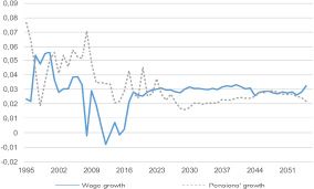
Figure 1 shows the evolution of wages and pensions over recent decades and their projected growth rates. The average growth rate of wages between 1995 and 2008 was 3.5% and their projected future growth is 3%. Remarkably, pensions have grown at a rate higher than that of wages: 4.7% between 1995 and 2008, which has been corrected for the period 2008–60 (with an average growth rate of 3.1%). The main reason for the past increase is the so-called substitution effect —new pensioners obtained systematically higher pay-outs. Moreover, the minimum pension has also grown at a rate above the average.
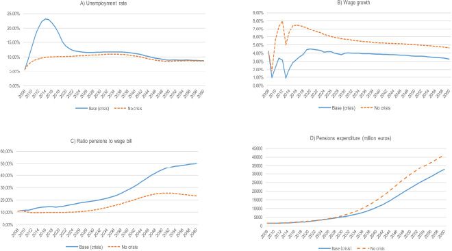
The year 2007 is selected as the base year to prevent projections being permanently affected by the 2008 economic crisis. However, at the same time, the effects of the crisis cannot be ignored. Hence, we opt for an ad hoc simulation of a reduction in the growth rate of wages and a temporary increase (decrease) in the job destruction (creation) rate. Given the uncertainty about the duration of the crisis, we assume a slow recovery ending in 2018. The changes observed in the job destruction and creation rates during the crisis (FEDEA, 2012) are applied when constructing the transition hazards (unemployment and re-employment) of our model from 2008 to 2018. An explanation of the overall effects of the crisis on sustainability and on job creation and destruction rates between 2008 and 2012 are provided in Appendix C.

Average wage and pension growth rates (1995–2060).
Sources: Annual Economic Database (1995–2008), European Commission and Spanish Social Security (2008–2060), authors’ calculations.
5.2 Behavioural responses to reform measures
We report the results obtained from simulating the effects of the 2011 pension reform (see Section 2 for more details) in which the baseline scenario includes behaviour and the impact of the crisis. Besides delaying the general age of retirement from 65 to 67, the rest of the measures aimed at boosting the system’s contributory nature, or the degree of proportionality between contributions and pensions, thus strengthening the Bismarckian nature of the system. This objective has been present on the Spanish reform agenda since first expressed in the 1995 Toledo Pact.7 Interestingly, such measures can have either positive or negative effects on pension rights. They have positive effects on sustainability and potentially positive effects on redistribution. Given that our analysis incorporates more than one dimension, we first present the effects of the behavioural reactions on the most relevant indicators. This allows us to test whether agents behave as expected. Second, the effects of the 2011 reform on both scenarios —with and without behaviour— are compared. Finally, the effects of the different measures of the 2011 reform are analysed separately for the behavioural scenario.
Figure 2 shows the pure effects of introducing behaviour into the retirement event. As expected, initial pensions are higher when individuals can react to financial incentives. Likewise, panel B of Figure 2 indicates that, when behaviour is considered, individuals tend to retire when the gains in entry pensions are higher and to delay retirement during years of crisis. This makes sense for several reasons. First, if we examine the model without behaviour we see that most of the variables —and with powerful effects as shown by the estimations— impel individuals to retire earlier. Only the most sophisticated indicators related to the financial incentives introduced in the behavioural model lead workers to consider the future benefits of waiting for a higher pension. Second, the effect of the crisis on working careers seems marked, pointing to the notable benefits to be gained from continuing to work after the crisis.
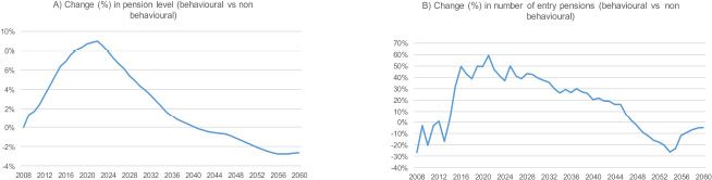
Behavioural versus non-behavioural model.

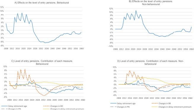
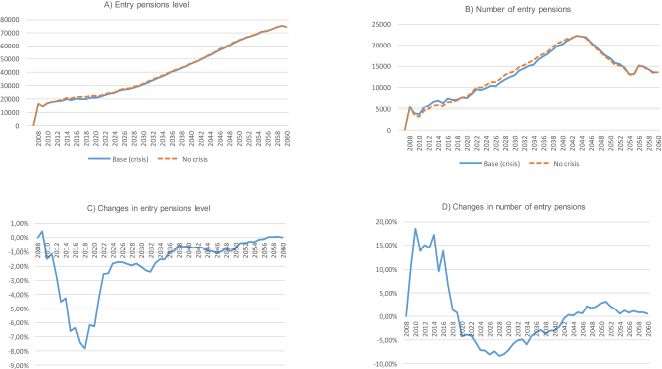
Effects of the 2011 reform on the level of entry pensions (% change).
We describe the effects of the 2011 reform in both scenarios —with and without behaviour— in Figures 3 and 4. Panels A and B of Figure 3 show the effects of the reform on the level of entry pension. In both scenarios, the reform is associated with an increase in initial pensions (until 2029 in the behavioural and until 2030 in the non-behavioural scenario). In the behavioural model, we observe a short period (2008–2010) of decrease that breakes the trend. We then observe a decrease in entry pensions that seems to be corrected at the end of the microsimulation period. Both the increase in entry pension associated with the reform and the further decrease are greater in the behavioural model, which is coherent with the results in Figure 2. Panels C and D detail the contribution of each reform measure. The reform in the number of years used to compute the BR (increasing gradually from 15 to 25) seems to account for the increase in pensions in both scenarios. This effect is surprising at first glance. The expected effect of this measure depends on the shape of the lifetime real earnings profile.8 If it is increasing, when the BR takes more years from the past this means a reduction in the wage level considered and, hence, a cut in pension rights. Yet, earnings do not always grow at the same rate across the life cycle. The typical profile can be expected to grow more at the beginning, to stabilise around the age of 50 and, thereafter, to remain constant or possibly worsen, if the career is interrupted by unemployment. Hence, the effect of this measure can be a small cut or even an increase in the pension benefit if wages are not growing in real terms. The unexpected increase in pensions observed during the crisis is probably due to the fact that the increase from 15 to 25 years meant adding years of contributions unaffected by the crisis.
The delay in statutory retirement from 65 to 67 does not result in a cut in entry pensions until approximately 2030. Before then, the effect is unremarkable. The change in p(n) means a decrease in the level of initial pensions, reaching almost 2% in the case of the non-behavioural and in the behavioural model. This average negative effect likely conceals positive and negative effects for those with different working careers. In general, reforms of p(n) have potential effects on redistribution. Nevertheless, in this particular case they are small, due to the scale of the reform. Changes in the incentives for delayed retirement are associated with higher pensions in both scenarios.

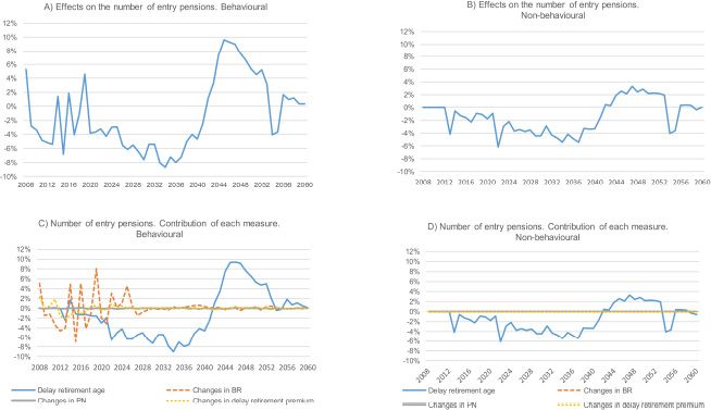
Effects of the 2011 reform on the number of entry pensions (% change).
Figure 4 describes the number of entry pensions. The 2011 reform produces an apparently erratic trend in this number in the behavioural scenario. The only measure that seems to incentivise people to retire earlier during the first years of the simulation is the change in the computation of the BR. This is consistent with the intuition explained above: if the sum of the earlier years of working history used to compute the average base are “better”, the incentives to continue working (probably with relatively lower wages) are weaker. The delay in the retirement age causes, as expected, fewer retirements during the first part of the simulation, but is offset during the period 2042–53. Unsurprisingly, the only measure that has an effect on the time of retirement in the non-behavioural scenario is the “compulsory” one: delay in retirement age from 65 to 67. In this scenario, agents are not allowed to use retirement time to react to the changes in financial incentives. Consequently, other measures produce no changes.

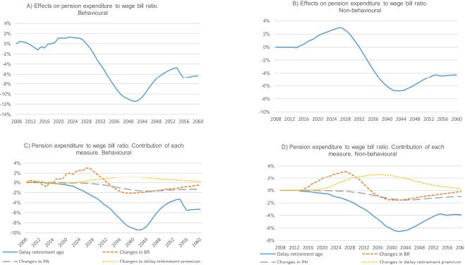
Effects of the 2011 reform on the pension expenditure to wage bill ratio (% change).
The most general indicator, which summarises the different effects of the pension reform, is the ratio between total pension expenditure and the wage bill. Figure 5 shows the percentage changes in this ratio and the contribution of each measure. In the behavioural scenario, the ratio falls due to the introduction of the reform over the whole period, except for the period 2014–32. As expected, the change in the computation of the BR is —except during the initial years— associated with a higher ratio, as is the increase in the retirement premium for delayed retirement, whereas the delay in retirement age cuts this ratio, and is the only measure that significantly improves sustainability (changes in p(n) operate in the same direction, but their effects are weak).
5.3 The role of demographics
Demographics play a key role in the evolution of the pension systems. Besides ageing, the role of the education transition (i.e., a progressively higher educational attainment) and the increase in female labour market participation are increasingly relevant. Below, to evaluate their respective roles, we present the results of two counterfactual scenarios.
5.3.1 Education
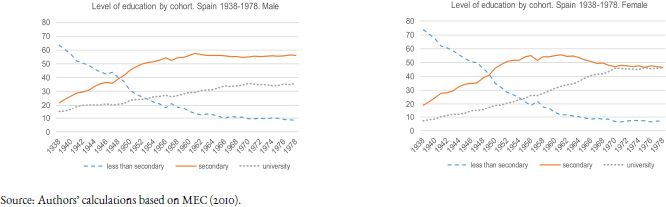
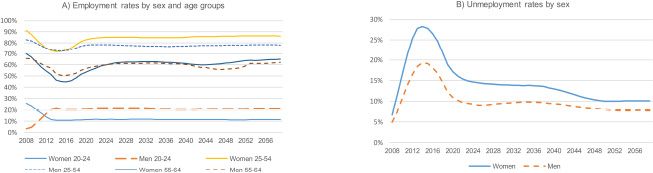
Educational attainment is modelled in two different ways: for individuals already in the starting population and born after 1978 (who supposedly have finished their studies by 2007, the year of the sample) the information is recorded as a variable; for future generations, the distribution of population by education level is imputed according to official data and projections from the Instituto de Evaluación, Ministerio de Educación y Ciencia (MEC). Figure 6 shows Spain’s education transition (ending with the cohort born in 1978), with rates of university studies close to 45% for women and 35% for men. Our projections assume these high rates will be maintained in the future (given that supposing further improvements would be unrealistic).

Educational attainment by gender.
Source: Authors’ calculations based on MEC (2010).
Yet, despite this increase in the educational attainment of Spanish youth, its impact on wages and future pensions is not direct as it is mediated by labour market performance. Indeed, it is quite plausible that the labour market will not translate this increase in human capital into better working careers (higher labour force participation and higher wages). In our model, educational attainment, labour force participation and working careers are closely linked so that a level of educational attainment is first assigned to individuals (as described above); second, entry contribution groups are assigned according to observed hazards by level of education and sex; and, finally, unemployment and re-employment hazards are held dependent on the level of qualification. Thus, the more highly educated rise faster to reach higher occupation levels and are more likely to end up in the highest contribution groups.
Figure 7 shows how, in the baseline scenario, the proportion of educated people employed in the highest contribution group increases with time, supposing an increase in the capacity of the labour market to absorb improvements in human capital. The only official data available on employment for those with tertiary education to contextualize our scenario come from de Estadística (2014) and Santiago, Brunner, Haug, Malo, and di Pietrogiacomo (2009). These reports contain employment information up to 2014 for those graduating four years previously. Yet, our scenario is coherent with these data sources, reporting employment rates in the highest contribution group of 19 and 22% for women and men, respectively.

Proportion of population with university studies employed in the highest contribution group.
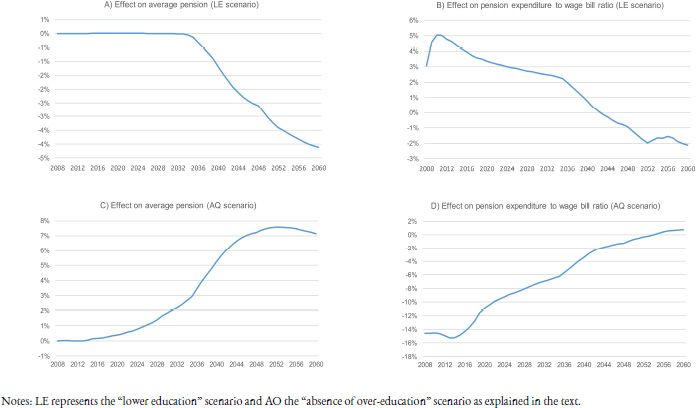
To verify the impact of changes in education on the pension system, two counterfactual scenarios are simulated. The first supposes that the observed education transition did not occur, so the education distribution of those born in 1950 (observed in our starting subsample) applies to all subsequent generations (lower education, LE-scenario). This distribution implies rates of 11, 41 and 48% for university, secondary and below secondary studies, respectively, for women, and rates of 15, 48 and 37% for men. In contrast, the second scenario supposes that the increase in human capital is fully translated into higher occupation rates in the highest contribution group, that is, the scenario supposes that all workers with university education rise to the highest contribution group in the second transition (absence of over-education, AO-scenario).
Not unexpectedly, the results of these two scenarios present opposing pictures of the average pension evolution and its relation to wages. Panels A and B in Figure 8 show the effects of lowering educational attainment on the average pension and the ratio of pension expenditure to the wage bill. During the first period of this projection, lower education levels translate into lower wages, weakening the sustainability of the pension system. After 2045, the situation is reversed, as less educated workers retire with lower pension benefits (lower wages during their careers results in lower pensions from 2035 on).
The effects of the second scenario point in the opposite direction and are more sizable (panels C and D in Figure 8). The “pure” effect of Spain’s education transition involves an increase in the average pension, reaching growth rates close to 8% in 2050. The initial improvement in the system’s sustainability is even more notable, with reductions in the ratio of total pension expenditure to total wages close to 16% during the initial period of simulation. As in the first scenario, the situation is reversed after 2045, when the more highly educated cohorts —who have been in the highest contribution group with the highest wage levels— retire.
5.3.2 Female labour participation
In the DyPeS model, labour force participation is the result of various interactions: entry hazards by education, sex and contribution group; changes in contribution groups by contribution group of origin and sex; and unemployment and re-employment hazards by sex and contribution group. The modelling is conducted using observed hazards for 2007. Insofar as no alignments are made in this baseline scenario to adjust results to any reference scenario, the resulting employment and participation rates are the “pure” result of interacting the increase in human capital with labour market transitions.

The effect of education on pensions (% change).
Notes: LE represents the “lower education” scenario and AO the “absence of over-education” scenario as explained in the text.
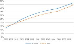
Before assigning individuals to a contribution group, DyPeS assigns them an educational level based on official data, capturing in the process the significant increase in Spain’s educational attainment. This increase in human capital has an effect on labour force participation. In particular, the increasing educational levels of women (surpassing those of men) have their counterpart in relatively high female employment rates (see panel A of Figure 9). While these rates are strongly affected by the increase in human capital and remain similar to or even higher than those for men throughout almost the whole period, unemployment rates also remain significantly higher for women (see panel B of Figure 9). This reflects the fact that women are more likely to be affected by periods of unemployment, although this is partly offset by their increasing labour force participation in the form of transitions from non-participation to employment (note, employment rates are calculated over the total population of young people, including non-participants, while unemployment rates are calculated considering only the active population).
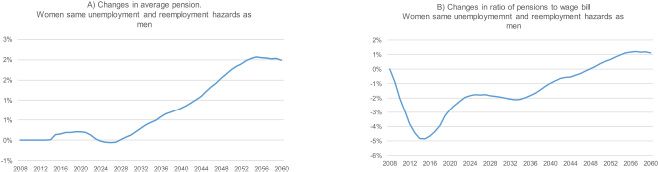
The impact of this situation is analysed in a hypothetical scenario in which women present the same unemployment and re-employment hazards as men. Figure 10 shows that the effects of this scenario on the pension system’s sustainability are sizable. However, while the impact on the average pension paid is only relevant at the end of the simulation period, the effect on the ratio of total pension expenditure to the wage bill (reflecting the higher contributions associated with increased female participation) are notable from the outset. As in the case of improved labour market performance, the situation is reversed at the end of the simulation, when women with longer careers (and higher average contributions) retire.

Labour force evolution (2008–2060). Baseline.

The effect of higher female participation on pensions (changes in %).
6. Final remarks
The sustainability of pension systems in most industrialised countries is threatened by demographic ageing. However, in parallel, other demographic characteristics are changing and may have a counter effect on sustainability. Two obvious examples are shifts in the labour market caused by an increase in the participation of older workers and women and the improvement in education levels. Similarly, the behavioural reaction of these heterogeneous agents to policy adjustments may well modify the impact of policies.
As such, there is an undoubted need for sound simulation models that can project pension expenditure and evaluate the effects of potential reforms. In this regard, the necessity of capturing the behaviour of agents that present different characteristics requires the use of microsimulation models. With the progressive availability of longitudinal microdata and enhanced computation methods, the most innovative models can aim at capturing the behavioural response of individuals to retirement incentives. In this paper, we have introduced individual behaviour into a dynamic microsimulation model applied to Spain (DyPeS). The retirement decision is modelled using a reduced-form survival model that provides information on retirement hazards. These are then introduced into the microsimulation model to estimate times of retirement. DyPeS is applied to a rich administrative dataset (the MCVL) produced by the Spanish Social Security. The model reproduces the main life-cycle events that affect pensions: birth, entry into the labour market, unemployment, retirement and death. DyPeS is a case-and population-based model, and was modelled in continuous time. It was implemented using ModGen, a programming language developed by Statistics Canada.
DyPeS allows us to simulate the 2011 measures reforming the Spanish pension system. Two of these aimed at increasing its contributory nature (by raising the number of years needed to compute the initial pension and by changing their weight in the formula, making it more proportional). A second measure aimed at reducing early retirement and promoting delayed retirement (by increasing the penalty in the case of the former and the premium in the case of the latter). Finally, the main measure was the delay to the general retirement age from 65 to 67. Our results show that accounting for individuals’ behavioural responses enhances projected pension system sustainability. Specifically, the total pension expenditure to wage bill ratio, which increases until 2036 in the non-behavioural model, would initially fall until 2022 and only increase in the period 2022–31. Interestingly, the delay in retirement age has the most significant effect on pension expenditure, while measures modifying the computation of the initial pension for new retirees have a limited impact.
The model also allows us to evaluate the impact of other demographic characteristics on pension system sustainability. Specifically, the role of changes in educational attainment and female participation can be analysed. In relation to the former, we examine two hypothetical scenarios, one that reverses the education transition and another that assumes all qualified workers find employment in the highest contribution group. Results show that education and, more specifically, the capacity of the labour market to absorb qualified workers, do matter. Higher levels of educational attainment mean higher wages in the short and medium term, reducing significantly the pension expenditure to wage bill ratio until 2050. Yet, they also imply higher pension benefits in the distant future, but with a limited impact on sustainability. In contrast, the lower education scenario produces a marked increase in the ratio until 2042, given the lower wages financing pensions. Sustainability only improves when the lower educated workers retire on correspondingly lower pensions.
In the case of female participation, we examine a hypothetical scenario in which women have the same unemployment and re-employment hazards as men. Again, the effects on pension sustainability are notable, showing that the labour market plays a critical role in the evolution of pension sustainability.
Footnotes
1.
The possibility of switching to a funded system is limited by the so-called transition problemml: the initial gift given to generations who did not contribute and received a pension now needs to be offset by a double burden on current workers, who need to maintain the old PAYG system and contribute to the new one. Some countries have opted for some kind of notional funding, which might be considered a more sophisticated way of introducing a defined-contribution system.
2.
Examples of use of DyPeS can be found in Fernández-Díaz, Patxot, and Souto (2013).
3.
Details about the reform of the Spanish pension system implemented in 2011 can be found in Section 2. The most significant measure was the delay in the general retirement age from 65 to 67.
4.
Contribution groups are classified by qualification level and contribution base thresholds: Group 1) Engineers, university graduates and senior management personnel; Group 2) Engineering technicians, experts and assistants with university degree, administrative and workshop managers; Group 3) Unskilled assistants, administrative Officials, subordinates, administrative assistants; Group 4) Unqualified part-time workers (first and second degree skilled workers, third degree skilled workers and specialists and unskilled labourers).
5.
The 2011 reform also announced the eventual introduction of a “sustainability factor” to cope with rising levels of life expectancy, albeit in a somewhat vague fashion. This was eventually regulated in 2013.
6.
For the sake of simplicity, we do not consider the possibility of an individual returning to the labour force after retirement, given the low incidence of this occurrence in Spain. In Spain, besides partial retirement, there are various legal pathways back into the labour force following retirement. However, it is still too early to evaluate the effects of these measures which, for the time being, have had very limited impact.
7.
The Toledo Pact, signed in 1995, by Spain’s main political forces, agreeing to a set of recommendations to underpin reforms guaranteeing the sustainability of the Social Security System.
8.
The relevant magnitude is real wages (and, hence, contributions), as the formula to compute BR updates wages to include inflation two years prior to retirement.
Appendix
A. A Retirement decision estimations
Hazard rate model for retirement with SSW incentives.
| Men Hazard ratio |
Standard error | Women Hazard ratio |
Standard error | |||
|---|---|---|---|---|---|---|
| Age | 154.48 | 47.83 | ** | 9.909 | 4.223 | ** |
| Age Sq. | 0.952 | 0.002 | ** | 0.971 | 0.003 | ** |
| Secondaty studies | 0.916 | 0.028 | ** | 0.890 | 0.045 | ** |
| Universitary studies | 0.943 | 0.032 | * | 0.966 | 0.062 | |
| First year retired | 4.176 | 0.164 | ** | 3.805 | 0.409 | ** |
| Unemployed | 0.673 | 0.026 | ** | 0.726 | 0.038 | ** |
| Unemployed benefit | 0.287 | 0.069 | ** | 0.222 | 0.072 | ** |
| Wage (1000 € change) | 0.910 | 0.000 | ** | 0.943 | 0.000 | ** |
| SSW | 1.000 | 0.000 | ** | 1.000 | 0.000 | ** |
| PV(a) | 0.994 | 0.000 | 1.000 | 0.000 | ||
| Time to PV | 0.899 | 0.015 | ** | 0.892 | 0.022 | ** |
| Age at PV | 1.002 | 0.000 | ** | 1.002 | 0.000 | ** |
| Replacement rate | 0.972 | 0.015 | * | 1.151 | 0.037 | * |
| Minimum pension | 1.391 | 0.050 | ** | 2.131 | 0.101 | ** |
| Months since elegible (log) | 1.937 | 0.031 | ** | 1.554 | 0.037 | ** |
| BR (1000 € change) | 1.002 | 0.000 | ** | 1.000 | 0.000 | ** |
| Unemployment rate | 1.009 | 0.002 | ** | 1.018 | 0.004 | ** |
| Constant | 0.000 | 0.000 | ** | 0.000 | 0.000 | ** |
-
(a)
Base category: less than secondary.
-
(b)
**Significant at 5º% level.
-
(c)
*Significant at 10º% level.
In this appendix we show the results of considering a model that includes Social Security Wealth (SSW) and Peak Value (PV) as main financial incentives. These variables are commonly used in the literature (Gruber & Wise, 2005) and particularly in previous studies for Spain (Sánchez, Argimón, Botella, & González, 2013). These authors use SSW, the Social Security Accrual (SSA) and PV and find that all the coefficients of these social security variables are statistically significant with the expected sign. Increases in the total present value of the flow of pensions that a person will receive from the year she retires to the year she dies, i.e. a rise in SSW, increase the hazard. Increases in the difference of this amount derived from postponing the retirement (either one or more years) reduce the hazard, irrespectively of whether SSA or PV is used to capture the substitution effects. By contrast, after controlling from other variables we find that the effects of the SSW and PV variables are very weak, being non-significant in the case of the PV. Hence, we opted for discarding this model and used the one explained in Section 3 to describe the social security incentives involved in the retirement decision. Two different kinds of reasons might explain why our results differ from those found in Sánchez et al. (2013): some related to the data employed and others related to the model. First, there are differences in the subsamples employed. Sánchez et al. (2013) use a subsample of people entitled to a pension benefit and aged from 60 to 70 in 2006. Our period of reference is longer (2005 to 2010) and includes people aged from 60 to 75. That is to say, we observe retirement transitions occurring between 2005 and 2010 and not only in 2006. In this respect, the inclusion of three years affected by the economic crisis may affect the retirement patterns observed. Second, the period discrete time-varying variable in Sánchez et al. (2013) is defined in years, and ours is defined in months. Finally, models are not identical. For example, Sánchez et al. (2013) use control variables —such as regional dummies— that we do not include in our model. Note that in our modelling framework we can only include the variables that we are going to reproduce for future periods in our microsimulation model.
B. Wage estimations
Table B.1 shows the wage estimations used in our microsimulation model. All the variables behave as predicted by the theory. Variables related to productivity —education, experience— increase wages, and more qualified and non-manual jobs are better paid. Also, wage increases with age but at a decreas- ing rate and immigrants are worse paid than Spaniards. We introduced cohort effects —assuming a linear relation— through the variable ‘year of birth’, whose impact on wages is strong and positive. This variable tries to capture changes (supposed to be improvements over time) in individual skills and productivity, mainly related to changes in education system and access to education, health sys- tem improvements with effects on individual health (and productivity).
Yearly wage estimations Dependent variable: yearly wage (full-time equivalent).
| Men Coef | Std. Err. | Women Coef. | Std. Err. | |||
|---|---|---|---|---|---|---|
| Past wage | 0.516 | 0.000 | ** | 0.560 | 0.000 | ** |
| Age | 802.42 | 1.783 | ** | 633.54 | 2.153 | ** |
| Age Sq. | −5.097 | 0.022 | ** | −4.022 | 0.027 | ** |
| Immigrant | −1846.89 | 9.804 | ** | −976.68 | 12.80 | ** |
| Secondary studies | 1022.91 | 5.031 | ** | 1059.16 | 5.946 | ** |
| University studies | 1686.27 | 8.564 | ** | 2366.83 | 8.063 | ** |
| Experience | 0.042 | 0.000 | ** | 0.051 | 0.000 | ** |
| Experience Sq. | 0.000 | 0.000 | ** | 0.000 | 0.000 | ** |
| Non-manual work | 1503.31 | 4.943 | ** | 1360.39 | 5.698 | ** |
| Qualified work | 3733.78 | 11.29 | ** | 3905.67 | 12.33 | ** |
| Year of birth | 355.12 | 0.314 | ** | 279.10 | 0.401 | ** |
| Unemployment rate | 27.13 | 0.459 | ** | 45.01 | 0.548 | ** |
| Constant | −714479.50 | 629.37 | ** | −563384.90 | 803.22 | ** |
-
(a)
Base category: less than secondary.
-
(b)
**Significant at 5º% level.
-
(c)
*Significant at 10º% level.
C. The effects of the economic crisis
As a result of changes in unemployment and re-employment rates —simulated following FEDEA (2012) unemployment triples, as panel A in Figure C.1 illustrates— Figure C.2 shows the effects of the current crisis on entry pensions (both number and level). The main driving force of the changes observed is the decrease in the pension level, due to poorer working careers. This effect is sizeable, starting during the crisis and reaching 30% for the cohort retiring in 2036. The amount of past years’ contributions considered to compute the basic pension amount (BR) being between 15 and 25, it is obvious that these cohorts are those most affected by the cut in wages and unemployment spells associated with the crisis. As a result, there is an impact on the time path of the number of entry pensions. The crisis produces a delay in retirement during the period 2013–2018, probably caused by the need to offset losses of potential pension associated with lower wages and less time worked. This delay in retirement during the crisis produces the opposite effect during the following years: from 2019 to 2026, we observe more retirements in the scenario with crisis than in the baseline one. All these results show that there is a reaction in retirement decisions due to the big movements in labour status that the current crisis produces. In a behavioural model such as the one considered here, agents can exit the labour market through early retirement, escaping penalties, and then avoid a higher reduction in entry pension level. As we will see in the next section it seems that, when behaviour is incorporated into the model, workers effectively tend to retire later, coping in this way with the effect of the crisis on their labour careers. As shown in panels C and D of Figure C.1, the total effect of the crisis in terms of increasing total expenditure and ratio of pensions to wage bill is huge, despite the sizeable delay in entry pensions shown in Figure C.2. It is mostly the consequence of the dramatic fall in wages due to the crisis, which has permanent effects (see panel B of Figure C.1) This sensitivity analysis shows the potentially strong impact of the crisis and illustrates the difficulties in projecting the future evolution of wages and in designing the interplay between the micro and macro modules of the model.

Effect of the current crisis on pensions (level and number).

Effect of the current crisis on other indicators.
D. Unemployment probabilities weighting expected pensions
Unemployment probabilities for people older than 58 (Logit model).
| Men Coef. | Std. Err. | Women Coef. | Std. Err. | |||
|---|---|---|---|---|---|---|
| Coef. | Std. Err. | Coef. | Std. Err. | |||
| Age | 3.070 | 0.472 | ** | 0.675 | 0.386 | * |
| Age Sq. | −0.025 | 0.004 | ** | −0.006 | 0.003 | * |
| Immigrant | −0.574 | 0.062 | ** | −0.070 | 0.0780 | |
| Secondary studies | −0.279 | 0.063 | ** | −0.146 | 0.066 | ** |
| University studies | −1.704 | 0.395 | * | −1.516 | 0.476 | ** |
| Experience | 0.011 | 0.006 | * | −0.018 | 0.005 | ** |
| Experience Sq. | −0.000 | 0.000 | * | 0.000 | 0.000 | ** |
| Non-manual work | −0.555 | 0.064 | ** | −0.208 | 0.050 | ** |
| Qualified work | 0.439 | 0.385 | 0.437 | 0.460 | ||
| Unemployment rate | 0.080 | 0.004 | ** | 0.0230 | 0.004 | ** |
| Constant | −94.45 | 14.599 | ** | −21.153 | 12.001 | * |
-
(a)
*Base category: less than secondary.
-
(b)
**Significant at 5º% level.
-
(c)
*Significant at 10º% level.
E. Robustness checks
E.1 Change in data period
Table E.1 shows the results of the estimation of model 1 (period 2005–10) vis-á-vis the one currently used in the microsimulation model (model 2, period 2005–2014). The results are quite robust in the case of men. There are no changes in the sign of the coefficients and the magnitudes are quite similar. However, the differences between the estimations in the case of women are remarkable. Whereas previously the effect of age had been linear and negative, it is now quadratic and strongly positive. In fact, the results are now similar to those for men. The reasons for this may be linked to the impact of the crisis (that is, more women needing to work longer). Also, the coefficient for unemployment changes its sign, due to extreme changes in the value of unemployment rates.
Retirement model 2005–2014 vs. 2005–2010.
| Men Model 1 | Model 2 | Women Model 1 | Model 2 | |||||
|---|---|---|---|---|---|---|---|---|
| Age | 21.22 | ** | 43.08 | ** | 0.829 | ** | 77.87 | ** |
| Age Sq. | 0.976 | ** | 0.972 | ** | – | 0.968 | ** | |
| Secondary studies | 0.973 | 1.050 | ** | 0.857 | 1.142 | ** | ||
| University studies | 1.152 | ** | 1.062 | ** | 0.932 | 1.271 | ** | |
| First year retired | 11.22 | ** | 2.042 | ** | 7.252 | ** | 2.545 | ** |
| Unemployed | 0.656 | ** | 0.313 | ** | 0.692 | ** | 0.000 | |
| Unemployment benefit | 0.156 | ** | 1.000 | * | 0.213 | ** | 1.000 | |
| Wage (1000 € change) | 0.992 | ** | 0.994 | ** | 0.992 | ** | 0.994 | ** |
| PV(a) | 0.953 | ** | 0.998 | ** | 0.899 | ** | 0.993 | ** |
| Time to max. pension | 0.995 | * | 0.930 | ** | 1.002 | 0.968 | ||
| Age at max. pension | 1.000 | * | 1.000 | 1.000 | 1.000 | |||
| Replacement rate | 1.074 | ** | 1.146 | ** | 1.131 | ** | 1.199 | |
| Minimum pension | 1.124 | * | 0.926 | ** | 1.438 | ** | 0.862 | ** |
| Months since eligible(log) | 1.329 | ** | 2.627 | ** | 1.476 | ** | 3.182 | ** |
| Unemployment rate | 1.012 | ** | 0.986 | ** | 1.012 | * | 0.991 | |
| Constant | 5454.00 | ** | 0.000 | ** | 6453.00 | ** | 0.000 | ** |
-
(a)
Base category: less than secondary.
-
(b)
**Significant at 5º% level.
-
(c)
*Significant at 10º% level.
-
(d)
Difference with respect to maximum pension, 1,000 € change.
E.2 Omitted variables problem
Health and marital status were omitted from the retirement model due to limitations in our data set. Although these variables are to some degree represented in the sample, the information is insufficient to be projected in the simulation model. First, the only indicator for health status in the Muestra Continua de Vidas Laborales (MCVL) is the degree of disability (expressed as a percentage). Second, as regards marital status, the survey only contains information about the number, age, and gender of cohabitants. It is therefore impossible to match couples in the dataset and, hence, to know their characteristics or gauge the effect of financial incentives for retirement on a joint decision. The MCVL is based on individual not household records. Fortunately, while far from perfect, this information does allow us to test for the importance of omitted variable bias.
As for the link between the omitted health variable and some of our included variables (such as, edu- cation) and its joint impact on retirement, the international evidence is abundant. However, studies of the Spanish case are scarce. No data base reports both health status and financial incentives to retire. In fact, the MCVL is the only work history database that includes a variable related to health status, namely, disability. Therefore, we have re-estimated the same model including this time the degree of disability and a dummy variable for disability. The results indicate that the inclusion of this variable does not alter substantially the impact of the other variables. Its impact on retirement is significant formen (reducing retirement hazards) but not for women. This finding is in line with that obtained by Sánchez et al. (2013) et al. (2013), who also use the MCVL to explain retirement behaviour and include a dummy variable for disability in their model. Those receiving disability benefits the year before re- tirement show a lower hazard, probably reflecting the fact that, besides having a poorer health, they will probably be the ones receiving retirement disability pensions when they turn 65, the only age at which pensions of this type can be awarded, so they will tend to wait until they reach that age.
In the case of marital status we also perform an estimation controlling for this omitted variable, to the extent that this is possible. Specifically, we include a dummy variable that takes a value of 1 if the individual lives with a person of a similar age. The results show that the effect of including this variable does not alter the impact of the other variables.
Inclusion of disability.
| Men Model 1 | Model 2 | Women Model 1 | Model 2 | |||||
|---|---|---|---|---|---|---|---|---|
| Disability degree | – | – | 0.993 | ** | – | – | 0.995 | |
| Dummy disability | – | – | 0.751 | ** | – | – | 0.841 | |
| Age | 43.08 | ** | 43.31 | 77.87 | ** | 78.16 | ** | |
| Age Sq. | 0.972 | ** | 0.972 | ** | 0.968 | ** | 0.968 | ** |
| Secondary studies | 1.050 | ** | 1.049 | * | 1.142 | ** | 1.143 | ** |
| University studies | 1.062 | ** | 1.061 | * | 1.271 | ** | 1.270 | ** |
| First year retired | 2.042 | ** | 2.042 | ** | 2.545 | ** | 2.542 | ** |
| Unemployed | 0.313 | ** | 0.315 | ** | 0.000 | 0.000 | ||
| Unemployment benefit | 1.000 | * | 1.000 | * | 1.000 | 1.000 | ||
| Wage (1000 € change) | 0.993 | ** | 0.993 | ** | 0.992 | ** | 0.992 | ** |
| PV(a) | 0.994 | ** | 0.994 | ** | 0.993 | ** | 0.993 | ** |
| Time to max. pension | 0.930 | ** | 0.930 | ** | 0.968 | 0.968 | ||
| Age at max. pension | 1.000 | 1.000 | 1.000 | 1.000 | ||||
| Replacement rate | 1.146 | ** | 1.147 | ** | 1.199 | 1.200 | ||
| Minimum pension | 0.926 | ** | 0.926 | ** | 0.862 | ** | 0.862 | ** |
| Months since eligible(log) | 2.627 | ** | 2.629 | ** | 3.182 | ** | 3.180 | ** |
| Unemployment rate | 0.986 | ** | 0.986 | ** | 0.991 | * | 0.991 | |
| Constant | 0.000 | ** | 0.000 | ** | 0.000 | ** | 0.000 | ** |
-
(a)
Base category: less than secondary.
-
(b)
**Significant at 5º% level.
-
(c)
*Significant at 10º% level.
-
(d)
Difference with respect to maximum pension, 1,000 € change.
Inclusion of marriage/partnership.
| Men Model 1 | Model 2 | Women Model 1 | Model 2 | |||||
|---|---|---|---|---|---|---|---|---|
| Married/partnership | – | – | 1.078 | ** | – | – | 1.005 | |
| Age | 43.08 | ** | 44.05 | ** | 77.87 | ** | 70.42 | ** |
| Age Sq. | 0.972 | ** | 0.972 | ** | 0.968 | ** | 0.968 | ** |
| Secondary studiesa | 1.050 | ** | 1.061 | ** | 1.142 | ** | 1.131 | ** |
| University studies | 1.062 | ** | 1.072 | * | 1.271 | ** | 1.265 | ** |
| First year retired | 2.042 | ** | 2.059 | ** | 2.545 | ** | 2.415 | ** |
| Unemployed | 0.313 | ** | 0.357 | * | 0.000 | 0.000 | ||
| Unemployment benefit | 1.000 | * | 1.000 | * | 1.000 | 1.000 | ||
| Wage (100 € change) | 0.994 | ** | 0.994 | ** | 0.993 | ** | 0.993 | ** |
| PV(a) | 1.000 | ** | 1.000 | ** | 0.999 | ** | 0.999 | ** |
| Time to max. pension | 0.930 | ** | 0.932 | ** | 0.968 | 0.984 | ||
| Age at max. pension | 0.993 | 0.994 | 0.994 | 0.994 | ||||
| Replacement rate | 1.146 | ** | 1.140 | ** | 1.199 | 1.210 | ||
| Minimum pension | 0.926 | ** | 0.941 | ** | 0.862 | ** | 0.880 | ** |
| Months since eligible(log) | 2.627 | ** | 2.716 | ** | 3.182 | ** | 3.058 | ** |
| Unemployment rate | 0.986 | ** | 0.987 | ** | 0.991 | 0.999 | ||
| Constant | 0.000 | ** | 0.000 | ** | 0.000 | ** | 0.000 | ** |
-
(a)
Base category: less than secondary.
-
(b)
**Significant at 5º% level.
-
(c)
*Significant at 10º% level.
-
(d)
Difference with respect to maximum pension, 1,000 € change.
F. Sensitivity analysis
Retirement decision (Probit model).
| Men Coef. | Std. Err. | Women Coef. | Std. Err. | |||
|---|---|---|---|---|---|---|
| Age | 3.594 | 0.144 | ** | 3.554 | 0.183 | ** |
| Age Sq. | −0.027 | 0.001 | ** | −0.027 | 0.001 | ** |
| Secondary studies | 0.041 | 0.021 | * | 0.152 | 0.028 | ** |
| University studies | −0.015 | 0.026 | 0.318 | 0.055 | ** | |
| First year retired | 0.834 | 0.055 | ** | 0.918 | 0.069 | ** |
| Unemployed | −0.937 | 0.364 | ** | |||
| Unemployment benefit | −0.000 | 0.000 | * | |||
| Wage (100 € change) | −0.000 | 0.000 | ** | −0.001 | 0.000 | ** |
| PV | −0.000 | 0.000 | ** | −0.001 | 0.000 | ** |
| Time to max. pension | −0.100 | 0.012 | ** | −0.064 | 0.017 | ** |
| Replacement rate | 0.384 | 0.073 | ** | 0.267 | 0.133 | ** |
| Minimum pension | −0.065 | 0.021 | ** | −0.163 | 0.027 | ** |
| Months since eligible(log) | 0.928 | 0.064 | ** | 0.904 | 0.077 | ** |
| Unemployment rate | −0.019 | 0.005 | ** | −0.016 | 0.007 | ** |
| Constant | −118.203 | 4.682 | ** | −118.817 | 5.989 | ** |
-
(a)
Base category: less than secondary.
-
(b)
**Significant at 5º% level.
-
(c)
*Significant at 10º% level.
G. Validation
Panels A and B in Figure G.1 show the evolution of average pensions and average entry pensions, both observed and in the model (behaviour and non-behaviour). Panel C and D present the ratio between the number of pensions/entry pensions and the population aged 65 or older. As expected, the be- havioural model reproduces more precisely the observed behaviour. Only for the ratio of new pen-sioners to population aged 65 or older the simulation describes a sizeable different pattern compared to the observed ratio. Nevertheless, this trend is corrected and, for the last year with available observa- tions (2016), there is no appreciable difference between the behavioural model and the actual rates.

Effect of the current crisis on pensions (level and number).
References
-
1
The retirement-health nexus: A new measure of an old puzzleJournal of Human Resources pp. 315–330.
-
2
The retirement incentive effects of Canada’s income security programsCanadian Journal of Economics/Revue canadienne d’economique 36:261–290.
-
3
Microsimulating the evolution of Italian pension benefits: The role of retirement choices and lowest pensions indexingLabour 17:139–173.
-
4
Labor force transitions of older married couples in germanyLabour economics 6:229–252.
-
5
Pension incentives and the pattern of early retirementThe Economic Journal 112:C153–C170.
-
6
Social security programs and retirement around the world: Micro-estimation499–578, In, Social security programs and retirement around the world: Micro-estimation, University of Chicago Press.
-
7
Microsimulation of pension reforms: ehavioural versus non-behavioural approachJournal of Pension Economics & Finance 9:583–607.
-
8
Evaluation of policy options to encourage welfare to workAustralian Economic Review 39:273–292.
- 9
-
10
Themes in the economics of aging311–354, In, Themes in the economics of aging, University of Chicago Press.
-
11
Los efectos económicos de la ley de consolidación de la seguridad social. perspectivas fnancieras del sistema de pensiones tras su entrada en vigorLos efectos económicos de la ley de consolidación de la seguridad social. perspectivas fnancieras del sistema de pensiones tras su entrada en vigor, Tech. Rep., Instituto Nacional de Estadística (Spanish Statistical Office).
-
12
What are the consequences of the awg-projections for the adequacy of social security pensions?., ... others , What are the consequences of the awg-projections for the adequacy of social security pensions?, Vol., 65, CEPS.
-
13
The 2012 ageing report: Economic and budgetary projections for the 27 eu member states (2010–2060)European Economy, Brussels (2 May 2012).
- 14
-
15
Dypes: A microsimulation model for the spanish retirement pension systemDocumento de Trabajo, 06.
-
16
Retirement incentives, individual heterogeneity and labor transitions of employed and unemployed workersLabour Economics 20:106–120.
-
17
International comparison of social security systems.Chicago: The University of Chicago Press.
-
18
Social security programs and retirement around the world: Fiscal implications, introduction and summarySocial security programs and retirement around the world: Fiscal implications, introduction and summary, Tech. Rep., National Bureau of Economic Research.
-
19
Evaluating the labor supply effects of alternative reforms of the Spanish pension systemsMoneda y Crédito: Revista de Economía 222:271–312.
-
20
Mandatory superannuation and self-sufficiency in retirement: An application of the APPSIM dynamic microsimulation modelSocial Science Computer Review 29:67–84.
-
21
Laborsimml: an agent-based microsimulation of labour supply–an application to italyComputational Economics 27:63–88.
-
22
A survey of dynamic microsimulation models: uses, model structure and methodologyInternational Journal of Microsimulation 6:3–55.
-
23
Sistema estatal de indicadores de la EducaciónMEC, Sistema estatal de indicadores de la Educación, Tech. Rep., Instituto de Evaluación, Ministerio de Educación y Ciencia.
- 24
-
25
Dynamic microsimulation: A methodological surveyBrazilian Electronic Journal of Economics, 4, 2.
-
26
Patents as options: Some estimates of the value of holding European patent stocks.National Bureau of Economic Research Cambridge, Mass., USA.
-
27
Should pensions be redistributive? The impact of Spanish reforms on the system’s sustainability and adequacy (Documento de Trabajo No. 2017/02)Fundación de Estudios de Economía Aplicada (FEDEA).
-
28
Optimal replacement of GMC bus engines: An empirical model of Harold ZurcherEconometrica pp. 999–1033.
- 29
- 30
- 31
-
32
>Pension reform in Norway: Microsimulating effects on government expenditures, labour supply incentives and beneft distribution (Discussion Papers No. 524)Statistics Norway.
- 33
-
34
Distributional effects of the forthcoming Finnish pension reform–a dynamic microsimulation approachInternational Journal of Microsimulation 8:75–98.
-
35
Micro simulations on the effects of ageing-related policy measuresEconomic Modelling 27:968–979.
-
36
An estimable dynamic stochastic model of fertility and child mortalityJournal of Political Economy 92:852–874.
- 37
-
38
Social security programs and retirement around the world: Fiscal implications, introduction and summarySocial security programs and retirement around the world: Fiscal implications, introduction and summary, (Tech. Rep.), National Bureau of Economic Research.
- 39
Article and author information
Author details
Acknowledgements
This research received institutional support from the European Commission through the Joint Programming Initiative "More Years Better Lives" and the Spanish Ministry of Economy, Industry and Competitiveness (grant agreement PCIN2016–151). Comments from two anonymous reviewers contributed to improve an earlier version of this manuscript.
Publication history
- Version of Record published: August 31, 2018 (version 1)
Copyright
© 2018, Patxot et al.
This article is distributed under the terms of the Creative Commons Attribution License, which permits unrestricted use and redistribution provided that the original author and source are credited.