Simulating the joint distribution of individuals, households and dwellings in small areas
- Netherlands Environmental Assessment Agency (PBL), Netherlands
Abstract
This article proposes a sample-based methodology for synthesizing individuals, households and dwellings in small areas, illustrated using a case study of Amsterdam. The method encompasses the following steps: first, individual- and household-level tables are created separately using Iterative Proportional Fitting (IPF). Second, synthetic individuals are allocated into synthetic households using a combination of sorting algorithms and mixed integer programming. As such, the synthetic households are adjusted to accommodate the synthetic individuals, ensuring a consistent joint distribution of individuals, households and dwellings in small areas.
1. Introduction
There is a growing interest in microsimulation models covering small geographical areas (Tanton, 2014). Such spatial microsimulation models attempt to solve the problem of lacking or non-representative data within small geographical areas, providing a ‘best guess’ of policy-relevant indicators at a small scale. For example, spatial microsimulation has been used to estimate smoking rates in zones within a city using knowledge about the composition of the population in these zones (Tomintz, Clarke, & Rigby, 2008). An important usage of the technique is synthetic reconstruction of population within small areas. The synthetic population is a key component of disaggregated models of travel- and residential energy use, used for spatially fine-grained scenario analysis or for predicting local impacts of policy interventions (Guo & Bhat, 2007; Muñoz & Peters, 2014).
One of the main usages of spatial microsimulation is reweighting of survey sample weights to reflect the population-composition of a small area and possibly new constraints (Ballas, Rossiter, Thomas, Clarke, & Dorling, 2005). The output of the reweighting is a weight matrix, reflecting the probability that a household or individual is located in a certain zone. A second main usage is synthetic reconstruction, which entails constructing full tables of synthetic households or individuals on the basis of the weight matrix.
Spatial microsimulation methods can be further classified into deterministic or probabilistic techniques. The most widely used deterministic technique is iterative proportional fitting (IPF — see Lovelace & Dumont, 2016). Despite its popularity, IPF has a number of limitations. First, non- xistent individual- or household-types in the seed data can lead to the so-called ‘empty cell problem’. Second, control variables need to belong to the same ‘universe’, meaning that IPF can not be directly used to synthesize individuals and households at the same time (Pritchard & Miller, 2012). The latter limitation is the focus of this paper.
A number of recent papers has proposed methods for generating synthetic individuals and households at the same time (Auld & Mohammadian, 2010; Ma & Srinivasan, 2015; Namazi-Rad, Tanton, Steel, Mokhtarian, & Das, 2017). For example Arentze, Timmermans, and Hofman (2007) develop a two-step approach, where a first IPF procedure is used to aggregate individual-level attributes to the household-level and a second IPF procedure is used to synthesize the household population. Ye, Konduri, Pendyala, Sana, and Waddell (2009) propose the method of Iterative Proportional Updating (IPU), whereby individual- and household-level weights are adjusted to match joint individual- and household-level constraints. However, in cases with large number of constraints, sample-based algorithms such as the IPU become prone to the empty cell problem and may not converge (Lenormand & Deffuant, 2012; Pritchard & Miller, 2012).
This paper provides a sample-based method for estimating the joint distribution of individuals, households and dwellings and we illustrate the methodology with a case study of Amsterdam. In a similar vein as Muñoz, Dochev, Seller, and Peters (2016), we aim to develop a realistic environment of the building stock and its resident population. This requires synthesizing a consistent population of individuals, households and dwellings. The structure of our household survey is such that we could potentially generate a population of households and individuals with IPU. However, as shown in Appendix A.1, using IPU we experience problems with convergence. To overcome the problems we instead create two tables: one with synthetic household and dwellings and one with synthetic individuals. The main contribution of this paper is a methodology for resolving inconsistencies between the resulting individual- and household-level tables.
We base the population synthesis primarily on IPF. The technique is well known for its numerical stability and algebraic simplicity, making it fairly intuitive and attractive to practitioners. Our strategy involves an additional step to allocate synthetic individuals to synthetic households. We opt for an approach similar to that discussed in Barthelemy and Toint (2013); namely to start allocating synthetic household heads, proceeding by allocating the remaining family members. However, Barthelemy and Toint (2013) construct households from the table of individuals, using a combination of maximum likelihood estimation and tabu-search optimisation. Consequently, the synthetic households are, in their case, already consistent with the synthetic individuals. Due to the large number of household- and dwelling-level constraints, we choose to start with two separate tables of synthetic households and individuals. Although these tables are internally consistent, they are not consistent with each other, meaning that the synthetic households can generally not accommodate the number of synthetic individuals. The inconsistencies between the individual- and household-level tables could therefore lead to non-allocated individuals or households without members. We solve this problem using mixed integer programming, adjusting the members of the synthetic households in such a way that the changes to the household composition are minimised.
Our methodology encompasses the following steps: first, we create separate tables of synthetic households and individuals using IPF. Next, we allocate synthetic persons into synthetic households using a combination of heuristic sorting algorithms and mixed integer programming. This allows us to adjust the synthetic households such that they accommodate the synthetic individuals, ensuring consistency between the individual- and household-level tables.
The paper is structured as follows: Section 2 presents the data used for the population synthesis; Section 3 discusses the proposed methodology; Section 4 shows the results of an internal validation and Section 5 concludes.
2. Data
The first key input to IPF is a (non-spatial) survey which is used to create a seed of individuals or households. In our case, we use two separate surveys: one capturing households and dwellings and another capturing individual people. The second key input is aggregate geographical data, which is used to create small area constraints. This section gives a description of the data sources used in the paper.
2.1 Survey data: Dutch mobility survey (OVIN)
The Dutch Mobility Survey (OVIN) is collected yearly by Statistics Netherlands (CBS). The goal of the survey is to provide adequate information on the daily mobility of the Dutch population. To this end, the movement behavior of the Dutch population is described by place of origin and destination, time of the carriage, means of transport used and reasons for travel. In addition, considerable attention is paid to the background variables for a particular movement pattern and choice of transport.
Each version of OVIN contains around 40,000 respondents, and CBS assumes that the survey covers 1.9% of total travelled kilometres in the Netherlands. Respondents are individual persons and not households, although the data set contains information about household-level variables for each respondent.
In this paper we use 7 versions of OVIN (2010–1016) to generate a seed of individuals, ignoring the location of residence of each respondent. Table 1 shows the variables we include in the seed of individuals.
Variables from OVIN and their levels.
| Variable | Levels | Explanation |
|---|---|---|
| ind_lmstatus | active, not-active | labour-market status |
| ind_ethn | Dutch, foreign | ethnicity |
| ind_income | high, low, mid | household income |
| ind_gender | man, woman | gender |
| ind_age | 00_14, 15_44, 45_64, 65_AO | age |
2.2 Survey data: Netherlands’ household survey (WOON)
The goal of the Netherlands’ Household Survey (WOON) is to gather information about the housing situation of the Dutch population and their living requirements and needs. The survey includes information about the composition of households, the dwelling and living environment, housing costs, living requirements and housing re-locations. Frequency is three-yearly. A minimum of 60,000 respondents have to be reached, as the survey should also provide reliable information on small geographical areas. In this paper we use two versions of WOON (2012 and 2015).
WOON contains a large number of variables about households and dwellings, and we have to make choices on which household characteristics to include. Firstly, included variables should cover basic demographic information and they must be associated with the outcome(s) of interest (Burden & Steel, 2016). Secondly, the variables need to exist in both the survey data as well as in the aggregate geographical data. Table 2 shows the dwelling- and household characteristics that are included in our analysis. WOON contains additional information about the number of household members by age. As has been discussed, this information, listed in Table 3, can not directly be used for a joint individual-household synthesis with IPF. However, by using information from Table 3, we can aggregate the household members to estimate the population in each small area, predicting the population of individuals from the synthetic households.
Household and dwelling characteristics from WOON.
| Variable | Levels | Explanation | ||
|---|---|---|---|---|
| dw_typei | rental, owner-occupied | dwelling tenure | ||
| dw_type2 | apartment, house | type of dwelling | ||
| dw_byear | before 1945,1945–1969,1970–1989,1990 and later | building year | ||
| dw_dheat | no, yes | district heating | ||
| dw_size | (6,51], (51,68], (68,89], (89,3e+04] | size (m2) | ||
| hh_age_h | 15_44, 45_64, 65_AO | age household head | ||
| hh_gender_h | man, woman | gender household head | ||
| hh_ethn_h | Dutch, foreign | ethnicity household head | ||
| hh_income | high, low, mid | household income | ||
| hh_lmstatus | active, not-active | labour-market status head | ||
| hh_type | single, w_child, wo_child | household type |
Information about household members from WOON.
| Variable | Levels | Explanation |
|---|---|---|
| n_00_i4 | numeric | members between 0 and 14 years |
| n_i5_44 | numeric | members between 15 and 44 years |
| n_45_64 | numeric | members between 45 and 64 years |
| n_65_AO | numeric | members 65 years and older |
| n_persons | numeric | number ofmembers |
2.3 The neighbourhood and district maps (Buurt en wijk kaarten)
The Neighbourhood and District maps from Statistics Netherlands contain digital geographical information as well as key figures for municipalities, neighbourhoods and districts (gemeente, buurt, wijk) in the Netherlands. Key figures include data on population and its composition; firms; housing stock; energy use; income and transport.
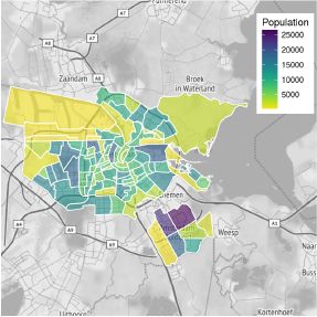
Figure 1 shows the population of each neighbourhood in Amsterdam. We use the 2014 classification of neighbourhoods, with a total of 98 neighbourhoods. Several of these neighbourhoods are industrial zones with negligible population, meaning that the number of neighbourhoods included in the analysis is 95. The total number of inhabitants is 810,825, distributed over 440,675 households. The plot shows that population is concentrated mainly around the centre and in suburbs in the south-eastern parts of the city.

Population in neighbourhoods in Amsterdam.
2.4 Additional data
The Neighbourhood and District maps only reports the mean value for a number of key variables of dwelling characteristics. In order to obtain a distribution for these variables we used additional open data sources. First, a distribution for the cadastral value of each neighbourhood was calculated from the 100x100m grid cell data from Statistics Netherlands. Second, categories of construction year as well as categories of dwelling size per neighbourhood were constructed on the basis of the Dutch Kadaster data. Table 4 lists all data sources and their usage.
Data sources and their usage.
| Source | Variables |
|---|---|
| OVIN 2010–2016 | Survey sample of individuals |
| WOON 2012 and 2015 | Survey sample of households and dwellings |
| Neighbourhood and District maps 2014 | Constraints on individuals, households and dwellings |
| 100x100m statistics | Constraint on cadastral value of dwelling |
| Dutch Kadaster data | Constraints on dwelling size and building year |
3. Population synthesis: Methodology
We use IPF to calculate neighbourhood-level weights for (i) individual respondents from the mobility survey OVIN and (ii) household respondents in the housing demand survey WOON, to fit the neighbourhood-level constraints. This results in separate tables of synthetic individuals and households consistent with the constraints. We proceed by allocating the synthetic individuals to the synthetic households. In this Section we first describe the generation of individuals’ and household tables including the constraints used. Next, we describe the methodology for allocating individuals into households.
3.1 Generating synthetic individuals and households using IPF
In general, the main output of a spatial microsimulation exercise is a table representing the most probable configuration of the population of small areas. The table is generated using a ‘seed’ of individuals or households from a survey and a number of constraints from geographically aggregated data. One of the most frequently used algorithms to generate the table is IPF. IPF is simple, computationally efficient, rigorously founded and it has a long history: it was first implemented by Deming and Stephan (1940), who estimated internal cells based on known marginals. The technique is also known as raking and is in practice identical to maximum entropy (Thissen & Löfgren, 1998). The output of IPF, when used in spatial microsimulation, is a series of non-integer weight matrices of a survey sample. Each cell in the matrix indicates how representative one survey respondent is of the real population within each geographical area. The weight matrix thus gives the most probable configuration of individuals in these areas.
The standard population synthesis using IPF involves two steps (Beckman, Baggerly, & McKay, 1996): the first step is to generate a joint multiway distribution of all relevant attributes of households or individuals. Next, persons or households are drawn from a seed of individual records in order to satisfy the distribution of attributes. The last step involves creating a list representing the synthetic population of individuals or households, using the weights generated by the IPF procedure. Since the weights are fractional, this step also involves integerisation of the weight matrix (Lovelace & Ballas, 2013).
Due to the popularity of IPF, there are several accessible and ready-to-use implementations of IPF in software programmes such as R (Lovelace & Dumont, 2016). In this paper the synthetic population of individuals is generated in R using the IPF procedure from the ipfp package (Blocker, 2016). As a consistency check, we repeated the exercise with the mipfp package (Barthelemy & Suesse, 2015) and results were identical.
As input for the synthetic population of individuals we used the respondent from the OVIN data set to generate the seed. The output of IPF in this case is a respondent-neighbourhood weight matrix consistent with the individual-level constraints for each neighbourhood. Constraints are the labourmarket status (ind_lmstatus), ethnicity (ind_ethnicity), gender (ind_gender) and age (ind_age) of each individual. The Buurt en Wijk Kaarten contains data for all these variables in percentages. To obtain the actual number we simply multiply the percentage with the number of individuals in the neighbourhood. The individual-level constraints, with their respective mean and standard deviation across neighbourhoods are presented in Table A.1 in the Appendix.
The synthetic household population is also generated with the IPF procedure from the ipfp package, using respondent from WOON as constraints. Dwelling variables include two types of classifications (dw_type1 and dw_type2), building year (dw_byear), size (dw_size), district heating (dw_dheat) and cadastral value (dw_value). For the sake of simplicity we ignore empty dwellings, setting the number of dwellings equal to the number of households. In addition to the dwelling-related constraints we also include constraints related to the household or to the household head; namely household income (hh_income), household type (hh_type), labour market status (hh_lmstatus), gender (hh_gender) and ethnicity of the household head (hh_ethn). Table A.2 in the Appendix shows the household- and dwelling-level constraints. Table 5 shows an example of five households from the sample seed derived from WOON. Note that the household-level constraints includes some information on the household head and the household composition.
Five households from the sample seed.
| hh 1 | hh2 | hh 3 | hh 4 | hh 5 | |
|---|---|---|---|---|---|
| dw_value | oo_199 | oo_199 | 2oo_299 | 2oo_299 | 00_199 |
| dw_typei | rental | owner | owner | owner | rental |
| dw_type2 | apartment | house | house | house | apartment |
| dw_byear | 1970–1989 | 1970–1989 | 1970–1989 | before 1945 | 1970–1989 |
| dw_dheat | No | no | no | no | no |
| dw_size | (68,89] | (89,3e+04] | (89,3e+04] | (89,3e+04] | (51,68] |
| hh_age_h | 65_AO | 65_AO | 45_64 | 45_64 | 65_AO |
| hh_gender_h | Man | man | man | man | woman |
| hh_ethn_h | dutch | dutch | dutch | dutch | dutch |
| hh_income | Low | low | mid | high | low |
| hh_lmstatus | not-active | not-active | active | active | not-active |
| hh_type | wo_child | wo_child | wo_child | wo_child | single |
| n_00_14 | 0 | 0 | 0 | 0 | 0 |
| n_15_44 | 0 | 0 | 0 | 0 | 0 |
| n_45_64 | 1 | 0 | 2 | 2 | 0 |
| n_65_AO | 1 | 2 | 0 | 0 | 1 |
| n_persons | 2 | 2 | 2 | 2 | 1 |
3.2 Allocating individuals to households
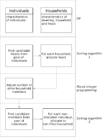
The overall approach for allocating individuals to households is summarised in Figure 2. The allocation of individuals into households consists of three parts: we first assign a household head from the individuals’ table to each household in the household table. This makes sure that each household has at least one member. Next, we adjust the numbers of remaining household members in the household table using mixed integer programming. Finally, we allocate the remaining household members to the adjusted households.

The overall population synthesis methodology.
3.2.1 Allocating household heads
In order to find household heads, we start with a pool of candidate individuals i = 1, ..., I with certain characteristics c and a pool of households h = 1, ..., H. Remember from Table 5 that the household survey WOON allows us to identify the following groups of characteristics of each household head: age, gender, ethnicity, labour market status (the levels of each group of characteristic can be found in the Table 2). Our strategy involves searching the pool of individuals whose characteristics match those of the household heads, allocating individuals to households using the matching characteristics.
More formally, in each neighbourhood, household heads are gathered in the matrix headh,c where rows indicate household ID and columns represent characteristics of the household head (for simplicity, the neighbourhood index is dropped). Similarly, individuals are gathered in the matrix indi,c. Each entry in headh,c and indi,c is a binary variable indicating whether the household head of household h or individual i has a specific characteristic c. The set c is a tuple, described in Table 6. The elements of c are defined in the second column of the table.
Characteristics used to match households and individuals.
| Dimension | Levels | Explanation |
| lmstatus | active, not-active | labour-market status |
| ethn | Dutch, foreign | ethnicity |
| gender | man, woman | gender |
| 00_14,15_44, 45_64, 65_AO | age |
The algorithm used for allocating household heads is described in Algorithm 1. We first initiate an empty matrix representing individuals per characteristics allocated into households alh,c = 0 and an indicator for successful match between an individual and households wdi,h = 0. We proceed by searching over all individuals who have matching characteristics with the household head in household h, updating alh,c when the first individual is found. In some cases there are no individuals left with fully matching characteristics. In those cases we search for individuals with matching characteristics in only three groups (age, gender, ethnicity). This way we make sure that each household has at least one member.
Allocation of household heads.
| 1: for all households do |
| 2: while |
| 3: for non-allocated individuals with matching characteristics do |
| 4: update alh,c = alh,c + indi,c |
| 5: set wdi,h = 1 |
| 6: end for |
| 7: end while |
| 8: end for |
3.2.2 Resolving inconsistencies between household and individuals’ tables
As shown in Table 5, WOON allows us to calculate the number of remaining household members by age, ethnicity and gender. We can express the amount of remaining household members with characteristic d in household h as the matrix hhh,d where d = c ∈ age, ethnicity, gender. Each entry in the matrix indicates the number of household members in h of category d. Therefore, the number of household members of characteristic d in household h is headh,d + hhh,d. Consequently,
The adjustment is formulated as a mixed integer problem where the (squared) adjustments of household members by characteristic are minimised. Adjustments are written as wh,d. In the case where wh,d ∈ {−1, 0, 1}, we have:
Intuitively, the mixed integer problem involves minimising the changes to the household composition (objective function) necessary to achieve consistency with the individuals’ table (constraints). The constraints in the the problem are (1) that same amount of adjustments are made across all groups of characteristics; (2) the amount of household members by characteristic d is non-negative and (3) the sum of household members by characteristic d is equal to the sum of individuals by characteristic d who have not been allocated as household head (indi,d for which wdi,h = 0):
The problem is solved for each neighbourhood separately, using the MOSEK solver in GAMS (MOSEK, 2018). We initially limit adjustments such that wh,d ∈ {−1, 0, 1}. In one small neighbourhood the problem is infeasible. In this cases we run the mixed integerisation problem iteratively, increasing the maximum value of adjustments until a solution is found.
3.2.3 Allocating the remaining household members
The adjustments made in the previous step ensure consistency between the household and individuallevel tables, meaning that there are enough ‘slots’ for allocating the individuals who have not yet been allocated as household heads. The algorithm used for the allocation of the remaining individuals (Algorithm 2), is similar to the algorithm used for the allocation of household heads. The algorithm starts with the pool of individuals who have not been assigned as household heads, and searches over households with available slots on characteristics matching those of the individual. For example, if individual i is a Dutch male between 15 and 44 years old, the algorithm will search over households with available slots on these characteristics. Once such a household is found, the number of household members in the household will be updated with the new member. In cases where there are no households with available slots on these matching characteristics, we simply allocate individuals to households who have an available slot.
Allocation of the remaining household members.
| 1: for non-allocated individuals do |
| 2: while |
| 3: for households with available slots on matching characteristics do |
| 4: set alh,d = alh,d + indi,d |
| 5: set wdi,h = 1 |
| 6: end for |
| 7: end while |
| 8: end for |
4. Internal validation of the results
This section presents internal validations of the household and individuals’ tables generated by IPF and of the allocation of individuals into households. As is common in the literature, we evaluate the fit of individual- and household-level tables using the correlation coefficient Pearson’s r and the root means square error (RMSE). The correlation coefficient shows the bivariate correlation between the fitted values and the constraints in each neighbourhood. It is thus a rough check of the numerical precision of the weight matrix per neighbourhood. RMSE gives further insight into the distribution of the residuals across constraints. We first calculate the residual ez,k of constraint k in neighbourhood z as the difference between the value of the constraint obsz,k and the simulated value simz,k. Then RMSE is calculated as follows:
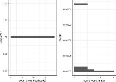
Since RMSE is scale-dependent, its value should be seen in light of the (mean) value of the constrain: the RMSE for a constraint with very large values across all neighbourhoods should be larger than the RMSE for a constraint with small values (see Table A.1 in the Appendix). However, in our case this is less of a problem. Figure 3, showing the correlation coefficient and the RMSE across all constraints for the individual-level table, reveals that all RMSE are very close to zero, suggesting a near perfect fit.

Correlation coefficient and RMSE of the individual-level table.
Due to the fairly large amount of constraints one might expect the fit of the household table to be worse than that of the individuals’ table. However, as Figure 4 shows, this is not the case: also here all RMSE values are very close to zero. From the internal validation we can conclude that the household- and individual-level tables both have a very good fit.
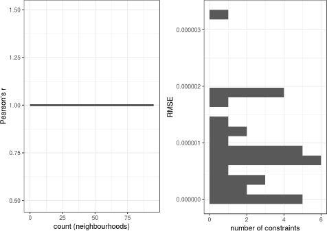
Correlation coefficient and RMSE of the household-level table.
As shown in the previous section, we are able to calculate the population of each neighbourhood by using information about household members from the household table. However, we also suggested that there were discrepancies between population from the household members and the individuals’ table. Obviously, if this were not the case, the mixed integer step would not be necessary.
We investigate whether there are discrepancies by calculating the percentage difference between the sum of unadjusted household members (membersz,h,d) and the sum of individuals in neighbourhood z. In essence, this amounts to checking whether the predicted population from the synthetic households is consistent with the constraint n_ind from Table A.1. The percentage difference is cal- culated as:
Figure 5 shows that there are indeed substantial discrepancies between the population from the household table and the population from the individuals’ table. The left panel, showing the density of diffz, gives evidence of positive deviations of up to 30%. However, the right panel, showing the cumulative density of diffz, suggests that the population is underestimated in a majority of the neighbourhoods.
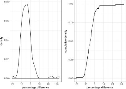

Neighbourhood population calculated from the households table relative to population calculated from the person-table.
We also run a x2 test of the improvement in fit by comparing the population from the unadjusted
Chi-squared test of neighbourhood population.
| X-squared | p-value | df | |
|---|---|---|---|
| unadjusted households | 617 | 0 | 94 |
| adjusted households | 0 | 1 | 94 |
In addition to ensuring correspondence between the household- and individual-level tables, our mixed integer programming aims at minimising changes to the household composition. It is therefore necessary to investigate whether we also achieve this goal. Figure 6 plots the frequency of households by number of members before (yellow) and after (purple) the adjustments. The figure suggests that our methodology leads to a slight increase in the number of households with one and three members relative to the unadjusted household.
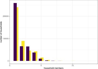

Number of members in the adjusted (purple) and in the unadjusted households (yellow).
Figure 7 plots the number of household members across age groups in the unadjusted (yellow) and adjusted (purple) households. It does not give evidence of very large changes to the age composition. Adjustments were primarily carried out in the age group 15 to 44.
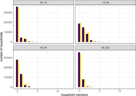

Number of household members by age in the unadjusted (yellow) and adjusted (purple) households.
Figure 8 plots the distribution of the percentage men and women per household across the unadjusted (yellow) and adjusted (purple) households. The figure shows that the share of households with an equal gender balance has been reduced, while there is a slight increase in the share of households consisting of only men. As above, the figure suggests that the adjusted households are fairly similar to the unadjusted households.
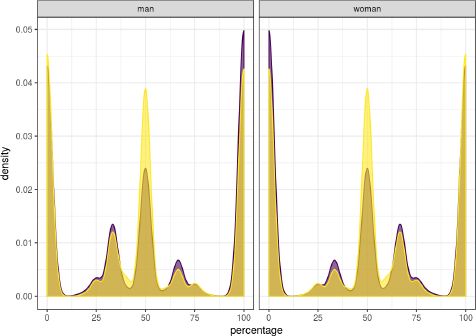

Percentage members gender in the unadjusted (yellow) and adjusted (purple) households.
5. Conclusions
This article reports on the creation of a spatial microsimulation model of Amsterdam. In the paper we have presented a methodology for joint synthesis of individuals, households and dwellings. Our proposed methodology encompasses the following steps: we first create separate household- and individual-level tables using IPF. Next, we allocate persons to households, resolving inconsistencies between the household- and individual-level tables using mixed integer programming. Our internal validation suggests that the method leads to a significant improvement in consistency between the two tables.
A major usage of spatial microsimulation is to construct a synthetic population for bottom-up models of mobility and residential energy use. These models are important tools in scenario analysis and policy analysis. However, this requires including variables that are relevant to mobility choices and energy use. In our case, the Dutch housing demand survey WOON provides detailed information about dwellings, households and persons. As such, one would be able to estimate energy use based on the household table alone. However, as evidenced by Figure 5, a population of individuals calculated from the household table deviates substantially from the population —in some cases by up to 30%. Such inconsistencies could potentially be solved by an algorithm such as the IPU. In fact, we first attempted to do so, but with limited success (see Appendix A.1). We suspect that the number or combination of constraints in our case are such that the IPU becomes vulnerable to the empty cell problem.
We provide, in our opinion, a fairly intuitive method for solving the problem of inconsistency. Granted, combining synthetic households and persons drawn from different surveys will always be difficult: a sample-free approach may be easier to implement and could indeed give a better fit (Barthelemy & Toint, 2013; Jeong, Lee, Kim, & Shin, 2016). We are of the opinion that a sample-based approach such as presented here is useful in practice. The survey used for creating the seed may well be used for purposes related to the spatial microsimulation exercise – for example to estimate the model used to predict a small-scale indicator. Such a direct connection between the population synthesis and the prediction is valuable in practical applications of spatial microsimulation.
Appendix
A.1 Results from IPU
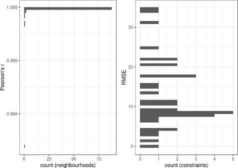
In this Appendix we construct a combined household-individuals’ table using the IPU algorithm implemented in the [a115]im[a80]op package (Templ, Meindl, Kowarik, & Dupriez, 2017). As mentioned, WOON also gives information about the number of household members by age category as well as the total household size. Since we have four age categories, we run the IPU with a total of 37 constraints: 32 for households and 5 for individuals. In the majority of the neighbourhoods, the algorithm did not converge. Figure A.1 shows the correlation coeffient and RMSE for the fit from IPU. The left panel suggests that problems with convergence are concentrated in a couple of neighbourhoods. The right panel of the figure suggests that the RMSE are orders of magnitude larger than in the IPF presented in the tables in the text. We believe that the problems we experience with IPU are related to the large number and composition of constraints.

Correlation and RMSE for the synthetic population created with IPU.
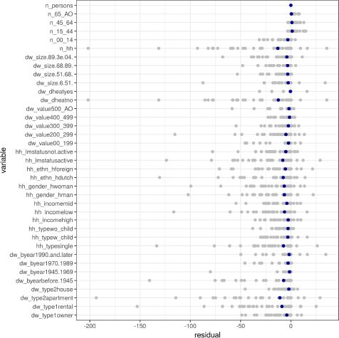
It is well known that the ordering of the constraints matter for both IPF and IPU: the best fit is likely to be seen with last constraint. Figure A.2 shows the residuals by constraints including the ordering of the constraints (the constraint on the top is the last). The blue dot shows the mean residual of each constraint. The figure clearly illustrates that the residuals are smallest for the last constraints (number of individuals) and that they in general are quite small for all individual-level constraints. The IPU algorithm seems to encounter difficulties with the constraints on the number of households, district heating and apartment.

Residuals by constraints for the synthetic population created with IPU.
A.2 Descriptive statistics of the constraints
Individual-level constraints.
| Variable | Mean | Standard deviation |
|---|---|---|
| ind_lmstatusactive | 494i | 3182.8 |
| ind_lmstatusnot-active | 3594 | 2605.4 |
| ind_ethndutch | 4211 | 2665.4 |
| ind_ethnforeign | 4324 | 3833.8 |
| ind_incomehigh | 1394 | ii84.4 |
| ind_incomelow | 4445 | 3i97.i |
| ind_incomemid | 2697 | i857.9 |
| ind_genderman | 4204 | 2762.4 |
| ind_genderwoman | 433i | 2865.2 |
| ind_age00_14 | i334 | ii08.0 |
| ind_age15_44 | 4099 | 2674.7 |
| ind_age45_64 | 2095 | i467.5 |
| ind_age65_AO | i007 | 776.5 |
| n_ind | 8535 | 56i8.7 |
Household-level constraints.
| Var | Mean | SD |
|---|---|---|
| dw_type1owner | 1247.2 | 861.0 |
| dw_type1rental | 3391.4 | 2278.5 |
| dw_type2apartment | 4074.4 | 2838.3 |
| dw_type2house | 564.2 | 885.5 |
| dw_byearbefore.1945 | 2070.9 | 2315.3 |
| dw_byear1945.1969 | 678.4 | 1343.6 |
| dw_byear1970.1989 | 778.4 | 1576.8 |
| dw_byear1990.and.later | 1111.0 | 1424.9 |
| hh_typesingle | 2536.6 | 1722.9 |
| hh_typew_child | 1160.1 | 913.4 |
| hh_typewo_child | 942.0 | 575.0 |
| hh_incomehigh | 747.2 | 592.1 |
| hh_incomelow | 2445.1 | 1739.0 |
| hh_incomemid | 1446.4 | 943.7 |
| hh_gender_opman | 2287.3 | 1469.7 |
| hh_gender_opwoman | 2351.4 | 1516.3 |
| hh_ethn_opdutch | 2331.3 | 1541.5 |
| hh_ethn_opforeign | 2307.4 | 1928.8 |
| hh_lmstatusactive | 2698.0 | 1730.9 |
| hh_lmstatusnot.active | 1940.7 | 1340.5 |
| dw_value00_199 | 1545.4 | 2169.1 |
| dw_value200_299 | 1965.0 | 1759.5 |
| dw_value300_399 | 646.1 | 893.8 |
| dw_value400_499 | 218.5 | 330.8 |
| dw_value500_AO | 263.7 | 661.3 |
| dw_dheatno | 4296.3 | 2805.9 |
| dw_dheatyes | 342.4 | 864.2 |
| dw_size.6.51. | 1135.7 | 1108.2 |
| dw_size.51.68. | 1226.5 | 966.2 |
| dw_size.68.89. | 1152.7 | 965.1 |
| dw_size.89.3e.04. | 1123.8 | 1131.9 |
| n_hh | 4638.7 | 2980.3 |
References
-
1
Creating synthetic household populations: Problems and approachTransportation Research Record: Journal of the Transportation Research Board 2014:85–91.
-
2
Efficient methodology for generating synthetic populations with multiple control levelsTransportation Research Record: Journal of the Transportation Research Board 2175:138–147.
-
3
Geography matters: Simulating the local impacts of national social policiesJoseph Rowntree Foundation, York.
-
4
Retrieved frommipfp: Multidimensional Iterative Proportional Fitting and Alternative Models, Retrieved from, http://cran.r-project.org/package=mipfp.
- 5
-
6
Creating synthetic baseline populationsTransportation Research Part A: Policy and Practice 30:415–429.
-
7
Retrieved fromipfp: Fast Implementation of the ITerative Proportional Fitting Procedure in C, Retrieved from, http://cran.r-project.org/package=ipfp.
-
8
Constraint Choice for Spatial Microsimulation568–583, Population, Space and Place, 22, 6, (PSP-14-0020.R2), 10.1002/psp.1942.
-
9
On a least squares adjustment of a sampled frequency table when the expected marginal totals are knownThe Annals of Mathematical Statistics 11:427–444.
-
10
Population synthesis for microsimulating travel behaviorTransportation Research Record: Journal of the Transportation Research Board 2014:92–101.
-
11
Copula-Based Approach to Synthetic Population GenerationPLOS ONE 11:1–28.https://doi.org/10.1371/journal.pone.0159496
-
12
Generating a synthetic population of individuals in households: Sample-free vs sample-based methodsGenerating a synthetic population of individuals in households: Sample-free vs sample-based methods, arXiv preprint arXiv:1208.6403.
-
13
‘Truncate, replicate, sample’: A method for creating integer weights for spatial microsimulationComputers, Environment and Urban Systems 41:1–11.
- 14
-
15
Synthetic Population Generation with Multilevel Controls: A Fitness-Based Synthesis Approach and ValidationsComputer-Aided Civil and Infrastructure Engineering 30:135–150.
-
16
The MOSEK optimization softwareMOSEK, The MOSEK optimization software, Retrieved from, http://www.mo[a115]ek.com.
-
17
Constructing a synthetic city for estimating spatially disaggregated heat demandInternational Journal of Microsimulation 9:66–88.
-
18
Constructing an Urban Microsimulation Model to Assess the Influence of Demographics on Heat ConsumptionInternational Journal of Microsimulation 7:127–157.
-
19
An unconstrained statistical matching algorithm for combining individual and household level geo-specific census and survey dataComputers, Environment and Urban Systems 63:3–14.
-
20
Advances in population synthesis: Fitting many attributes per agent and fitting to household and person margins simultaneouslyTransportation 39:685–704.https://doi.org/10.1007/s11116-011-9367-4
-
21
A review of spatial microsimulation methodsInternational Journal of Microsimulation 7:4–25.
-
22
Simulation of Synthetic Complex Data: The R Package simPopJournal of Statistical Software 79:1–38.https://doi.org/10.18637/jss.v079.i10
-
23
A new approach to SAM updating with an application to EgyptEnvironment and Planning A 30:1991–2003.
-
24
The geography of smoking in Leeds: Estimating individual smoking rates and the implications for the location of stop smoking services341–353, The geography of smoking in Leeds: Estimating individual smoking rates and the implications for the location of stop smoking services, Area, 40, 3.
-
25
A methodology to match distributions of both household and person attributes in the generation of synthetic populationsIn, 88th Annual Meeting of the Transportation Research Board, Washington, DC.
Article and author information
Author details
Acknowledgements
The research leading to this paper has been carried out under the Horizon 2020 project Clair-City. This project has received funding from the European Research Council (ERC) under the European Union’s Horizon 2020 research and innovation programme. Hans van Amsterdam (PBL) helped with collecting the Dutch cadaster data. The paper has benefited from comments from consortium members and from colleagues at PBL.
Publication history
- Version of Record published: August 31, 2018 (version 1)
Copyright
© 2018, Husby et al.
This article is distributed under the terms of the Creative Commons Attribution License, which permits unrestricted use and redistribution provided that the original author and source are credited.