The distributional impact of VAT reduction for food in Hungary: Results from a Hungarian microsimulation model
- National University of Ireland, Ireland
- University of Canberra, Australia
- Corvinus University of Budapest, Hungary
- Hungarian Academy of Sciences, Hungary
Abstract
In this paper we illustrate how the incorporation of behavioural responses and dynamic effects alters the conclusions of static household microsimulation models on the distributional impacts of economic policies. Based on Hungary’s Household Budget and Living Conditions Survey, we model household consumption using the demand system approach of Creedy, 1998. This method makes it possible to obtain reasonable price elasticity estimates of consumption from cross-sectional data by combining them with Frisch-parameter values obtained from cross-country studies. With this consumption module, we simulate the distributional impacts of a hypothetical food VAT rate change in Hungary and show how the static and behavioural impact estimates differ according to income decile. We examine the sensitivity of our results to the choice of the country-level Frisch-parameter and to a realistic allowance for household-level variation in the Frisch-parameter.
1. Introduction
Hungary, a Central European member state of the European Union with about 10 million inhabitants, has the highest VAT rate in the world at present with 27%, although a reduced rate of 18% applies to some food products. There is a continual debate about the necessity for and possible effects of a reduction in the VAT rate for all food products. The rate for certain meat products was decreased in 2016, and there are plans for further reductions for other food products. Additionally, VAT counts for 24% of total government revenue, higher than the OECD average (see OECD, 2016). VAT policy is an important issue for decision-makers, since almost one-third of the population of Hungary is at risk of poverty according to Eurostat, 2014.1 Furthermore, a quarter of the population is materially deprived. The social benefits of a possible VAT rate reduction for food have to be set against the fiscal effects of such a decision. The present paper examines this issue by means of microsimulation.
The government of Hungary launched the Zoltán Magyary Programme in 2010 in order to improve the efficiency of the Hungarian public administration. One of the elements of the Programme was the introduction of compulsory regulatory impact assessment (RIA). This type of ex-ante estimation of the impacts of bills and the monitoring of laws in force needs appropriate information systems and analytical tools. The economic and social impacts of changes in the taxation, social security and benefit systems can be quantified successfully by microsimulation models, therefore it is nowadays a routine practice to apply such models in the decision-making process in many countries in both the developed and the developing world. In this paper, we present simulation results to demonstrate how the incorporation of behavioural and dynamic features alters the distributional impacts of changes in tax policies. A general reduction of the VAT rate on food products is examined.
The paper is structured as follows. Section 2 presents background information on VAT in Hungary. Section 3 is devoted to the presentation of the methodology including some specific models developed in the context of Hungary. The estimation results for expenditure and price elasticities are discussed in Section 4. Section 5 summarises the simulations, showing how the behavioural effects may change the VAT burden of the different income deciles, and includes robustness checks. Finally, conclusions are drawn in Section 6.
2. Background of the VAT analysis in hungary
VAT in the EU member countries is regulated by a directive, with which the national regulations should be compatible, but there is a certain degree of freedom for the specific application of VAT in each country. According to the directive, the standard rate of VAT should be at least 15%, while at most two reduced rates can be applied for certain groups of goods and services. Correspondingly, the Hungarian standard VAT rate was able to remain at 25% when the country joined the EU in 2004, however, the two reduced rates in place at that time were raised from 0% to 5% and from 12% to 15%, respectively (exports are exempt from VAT). The VAT of certain products changed at the same time. The most important change occurred for electricity, for which VAT increased from the reduced rate of 12% to the standard rate of 25%. The rates were changed many times after 2004. The standard rate was reduced by 5 percentage points in 2006 as a part of an expansionary, demand-boosting fiscal policy. However, this policy resulted in high budget deficits (9.3% of GDP in 2006) and, correspondingly, a drastic increase in government debt. Because of the earlier expansive fiscal policy, the global financial crisis had severe consequences in Hungary from the end of 2008. The standard VAT rate was raised again up to 25% in 2009 as a part of fiscal consolidation, while the two reduced rates became 5% and 18%. This increase was introduced in July 2009, within the calendar year, since it became apparent that the original central budget planned for 2009 could not have been fulfilled. The standard rate increased further in 2012 and is now 27%, the highest VAT rate in the world. Figure 1 shows the rates in the OECD countries.
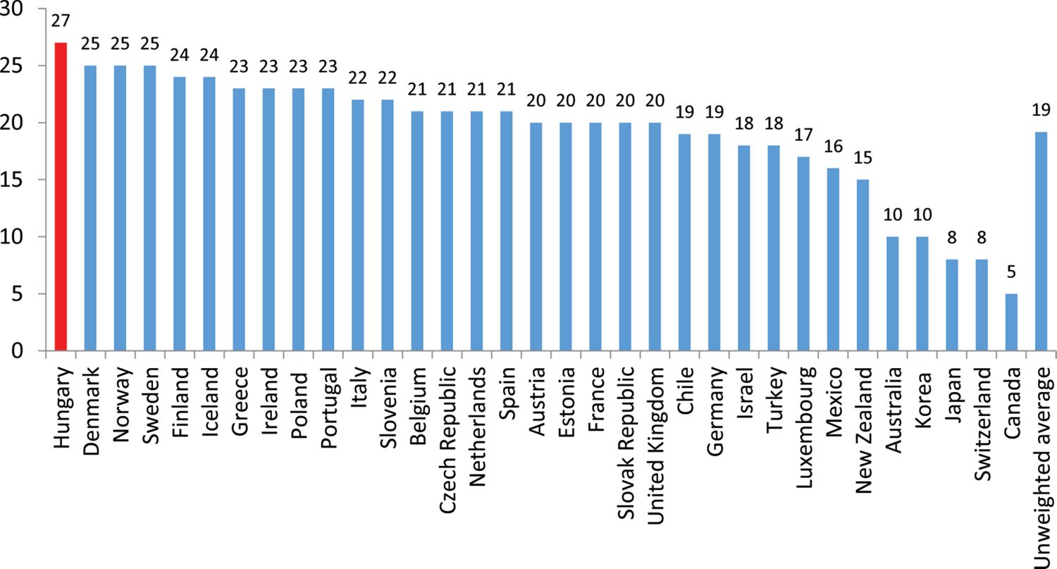
Standard VAT rates in the OECD countries (%).
Source: OECD, 2014.
In Hungary, the VAT burdens only final consumers. This means that in every phase of production, transportation and trade, the VAT should be paid for goods and services within the domestic territory and after importation, but all economic agents who are not final consumers may claim a VAT refund (this is the invoice method, i.e. the invoice is the basic document for exercising the right to claim a refund).
The relatively high VAT rate has certain advantages. According to economic theory and empirical evidence, high corporate income taxes are considered the most harmful to growth, since they may hurt business activities. High personal income taxes may reduce labour supply and discourage savings (the source of new investments), which are taxed twice: once as personal income and second as the yield of saving. Therefore, there are suggestions that the weight of consumption taxes should be relatively high in a growth-oriented tax mix (see for example OECD, 2010). This is the case in Hungary, where VAT is now the highest revenue item of the central government. In Hungary, an additional argument for the gradual increase of the VAT rate has been that there is less space for tax avoidance and tax evasion in VAT than, for example, in personal income tax. (For a discussion of tax evasion in Hungary see, for example, Benedek, Elek, & Köllő, 2013). However, the exceptionally high 27% VAT rate resulted in new types of tax evasion in certain industries, such as in personal services.
Another disadvantage of the high VAT rate is that the relative burden for lower income households is greater as a consequence of their high consumption rate, which may lead to an increase in social inequalities. Several studies discuss this regressive nature of indirect taxes: for example Ruiz and Trannoy (2008) and Decoster, Loughrey, O’Donoghue, & Verwerft (2010) examine this using microsimulation models. The distributional impacts of the indirect tax system have also been examined, for example, by Newbery (1995) and Newbery and Révész (1997) for the United Kingdom and for Hungary, although their analysis was not based on microsimulation. Tamaoka (1994) discusses the regressivity of VAT for Japan, a developed country, while some recent papers such as Jansen, Stoltz, and Yu (2013), Hanni, Martner, and Podestá (2015) and Fu (2016) examine this phenomenon specifically in certain developing market economies (see also their references). Gastaldi, Liberati, Pisano, and Tedeschi (2017) use microsimulation to analyse the distributional implications of the VAT, relying on the concept of Gini elasticity.
Decision-makers in Hungary intended to create a tax mix characterized by relatively high VAT and relatively low personal income tax (PIT) rates, since they expected that lowering the PIT rate —and consequently the tax wedge— would increase the competitiveness of domestic firms. However, the reduction of the PIT rate was carried out by a flat tax reform in 2011, which further increased inequalities (see Cserháti & Takács, 2011 and Cserháti, Keresztély, & Takács, 2012 for impact assessments).
Similarly to other countries, Hungary tends to apply reduced VAT rates primarily for utilities and basic food items that have a relatively high share in the consumption of the poorest strata. The aim of these reduced rates is to improve the situation of the poorest households that have low levels and a particular structure of consumption, than to remove the above mentioned regressive nature of VAT. Different industries also advocate for having lower rates applied to their goods and services, hoping that lower prices may increase demand for their output. According to current regulations, certain food products, cultural and tourist services are taxed at a reduced 18% VAT rate. The rate is 5% for some medical and food products, some cultural events and district heating. Finally, certain services (e.g. medical, cultural and social) are exempt from the VAT.2
Currently, there are no plans to change the general structure of taxation in Hungary; the VAT is expected to remain relatively high, but certain products may get into the reduced rate group or the VAT-exempt group in the near future. The possible changes are expected to concern those goods and services that have large weights in the consumption of households with relatively low disposable income. Since the controlled prices of household energy (gas and electricity) have recently decreased substantially, the proposed reductions of the VAT rate for some products may focus on food products. Therefore, in the present paper, we simulate the effects of VAT reductions on food: reducing rates for those with 18% tax down to 0% and those with the standard 27% down to a reduced 5%. This question is quite relevant because some types of food (milk, eggs and poultry) have indeed moved to a 5% VAT rate from the 1 January 2017. The simulation yields both the change in consumption of various consumption categories on the micro level and the change in budget revenues at the macro level. Even if the price elasticity of food products is relatively small, we may expect significant changes in the structure of final household consumption, if the change in these products’ specific VAT rates is large enough.
3. Methodology
3.1 International literature
Our main purpose is to quantify the impacts of a possible VAT rate change on different social strata, primarily on the different income deciles. This question can be answered effectively by microsimulation techniques. Many analyses for VAT reform utilise simulation models based on macro data, the computable general equilibrium (CGE) model being one of the most popular choices. Macro-models themselves can show only the effects on macro-indicators like GDP and employment (see, for example, Jackman, Layard, & Nickell, 1996; European Commission, 2006). Bye, Strøm, & Åvitsland (2012) estimated the welfare impact of VAT reform in Norway using a CGE model, Narayan (2003) analysed the macroeconomic impact of VAT reform in Fiji and Ye, Chang, Enhui, & Ming (2010) examined the employment impact of VAT reform in China. CGE models incorporate the potential behavioural responses of the assumed agents and are often used to estimate the fiscal impact of a policy nationwide. The models, however, are often insufficient in understanding the distributional effects of a reform. The limited number of representative households in CGE means that it cannot adequately capture the heterogeneity of the population and cannot answer in detail one of the most frequently asked policy questions — who wins or loses from reform.
Microsimulation models, on the other hand, are often used for distributional and win-lose analyses of a reform (see, for example, Sutherland, 1995; Li, & O’Donoghue, 2013; Li, O’Donoghue, Loughrey, & Harding, 2014; Figari, Paulus, & Sutherland, 2015 for surveys). Although traditionally focused on direct taxation issues, it is possible to extend the models to the analysis of indirect taxation. VAT, as one of the most important sources of indirect taxation, has been analysed in a number of papers using the microsimulation approach (e.g. Decoster et al., 2010; Decoster, Loughrey, O’Donoghue, & Verwerft, 2011; Decoster, Ochmann, & Spiritus, 2014; O’Donoghue, Baldini, & Mantovani, 2004; Capeau, Decoster, & Phillips, 2014 using EUROMOD; Abramovsky, Attanasio, Emmerson, Phillips, & Paez, 2010 using MEXTAX; and Siemers, 2014. Compared to CGE modelling, microsimulation models allow a much greater heterogeneity of responses among the population — avoiding the representative household assumption. Such models can be effectively used for estimating the distributional impact of a targeted VAT reform.
It is worth highlighting a number of modelling issues from these earlier papers on VAT microsimulation. Decoster et al. (2011) simulated a tax shift from labour to consumption for four European countries (including Hungary) in the EUROMOD framework. Similarly, Decoster et al. (2014) demonstrated the integration of VAT into EUROMOD in the Belgian and German cases. Instead of the application of price elasticities, the consumption equations in that paper are estimated as a regression function of disposable income and household-specific characteristics. Another VAT analysis for Germany using a general microsimulation model is presented by Siemers (2014), who discusses the treatment of hidden and shifted VAT (i.e. when the VAT cannot be claimed for an exempt good or service, although their inputs are not exempt); see also Gottfried and Wiegard (1991). In the Siemers (2014) paper the price elasticities for the poor and the rich are taken from the literature, not estimated. The simulations for different price elasticities show that the budget effects are susceptible to these elasticities.
It is clear from the above papers that a crucial issue in VAT microsimulation is the treatment of behavioural responses to price changes. Typical static microsimulation models do not consider the behavioural responses of households to changes in the regulation itself, as they assume that households do not alter their consumption behaviour after indirect tax changes (or their labour supply behaviour after income tax changes). These models, however, can be crude for analysing indirect taxation, as there can be significant behavioural adjustment given the price increases of goods. Previous literature using data for fifteen EU countries suggests significant consumption behavioural shifts in both the short and long term as a result of VAT changes (Alm & El-Ganainy, 2013). In the ECONS-TAX model used in the present paper we will model the consumption behaviour of households in response to price and income changes with a demand system method similar to that used by Creedy (1998). This method allows the estimation of price elasticities based solely on cross-sectional data, using exogenous information on the so-called Frisch-parameter.
3.2 Microsimulation modelling in Hungary and the ECONS-TAX model
Static microsimulation models have a long history in Hungary, where the first modelling attempts were made at the Hungarian Central Statistical Office in the 1980s (see Csicsman & Pappné, 1987 or for some results Redmond, 1999) and since then several institutions, including the Hungarian research institute TÁRKI (Szívós, Rudas, & Tóth, 1998), the Ministry of Finance (Benedek & Lelkes, 2005), the Office of the Fiscal Council (Benedek & Kiss, 2011) and the Hungarian Central Bank ‘MNB’ (Benczúr, Kátay, & Kiss, 2012) have used microsimulation techniques. The ECOS-TAX model, developed at the Ecostat Research Institute and later at the Office of Public Administration and Justice in Hungary, is also a static model (see Cserháti et al., 2012 for its description and Cserháti, & Takács, 2011 for its application to assess the distributional effects of a flat tax rate in Hungary).
The original static ECOS-TAX model was augmented by a dynamic labour market block and a consumption block to create the behavioural ECONS-TAX model in 2013. The main purpose was to build a model that is able to simulate the dynamic labour market and consumption impacts of changes in both income and indirect taxes, and can also be coupled with a macroeconomic model. In this paper we concentrate on the consumption block of ECONS-TAX. Its other modules (such as the micro-level stochastic simulation module for labour market transitions, the labour supply module and the macroeconomics module) and their interactions are presented by a flowchart in Appendix A.3
The starting point of the behavioural ECONS-TAX model is the micro-level database of the Household Budget and Living Conditions Survey (referred to as HKÉF, its acronym in Hungarian, below) of the Hungarian Central Statistical Office for 2011. This survey contains detailed information about the demographic characteristics, income and consumption of around 25,000 people in 10,000 households (or 0.25% of the Hungarian population). The income part of the survey is completely in accordance with the EU-SILC (European Union Statistics on Income and Living Conditions) standards, while the consumption part contains detailed household expenditures and purchased quantities for more than 500 categories of goods and services.
Due to possible underreporting bias, the HKÉF database (in common with other household surveys) underestimates the income of households compared with both personal income tax returns and the National Accounts. To correct for this bias and to make the data more appropriate for aggregate fiscal calculations, the database is matched with anonymised micro-level income data from personal income tax returns and with the wage survey database of the National Employment Service. Then, the survey sample weights are modified, and some minor income categories are imputed so that the aggregate incomes calculated from the survey are now equal to the aggregate income figures coming from other, macroeconomic sources. For details of the reweighting and imputing technique (see Cserháti et al., 2012). The behavioural modules of the ECONS-TAX model are estimated on this modified database. Some of our results have shown (see Cserháti, Keresztély, & Takács, 2015) that the correction may relevantly change the level of inequality indices (in particular the Palma index and the S80/S20), although their dynamics have not shown any significant change. Given a lack of reliable external consumption data, we do not explicitly correct for potential reporting bias of consumption although the reweighting procedure would implicitly retain the correlations across the reported attributes at the individual level.
The consumption module of the model receives net income at the household level and prices by consumption categories as inputs, from which the behavioural consumption equations— described in detail in the next subsection— yield the simulated net consumption of households.
3.3 Modelling behavioural responses of consumption tax
Consumption and VAT modelling in a microsimulation framework also has some history in Hungary. For instance, the TÁRSZIM model (Szívós et al., 1998) can be used to analyse indirect tax changes with and without behavioural responses, although price elasticities are not estimated within the model but can be exogenously determined by the user. Later, Cseres-Gergely and Molnár (2008) and Cseres-Gergely, Molnár, and Szabó (2016) estimated income and price elasticities in multi-product models for Hungary. Together with the international literature summarised in previous sections, this points to the importance of modelling behavioural responses of consumption in the microsimulation setting.
The main ingredients of the consumption module of ECONS-TAX are the estimated consumption functions, which come from a household demand system. Since the seminal article by Stone (1954) there has been widespread interest in choosing an estimable system of equations to represent household demand for various goods, the two most well-known approaches being the translog system of Christensen, Jorgenson, & Lau (1975) and the Deaton & Muellbauer (1980) almost ideal demand system (AIDS). Of these, the AIDS has proven to be more popular, because it permits exact aggregation over households and is easier to estimate. More recently, Banks, Blundell, & Lewbel (1997) presented a generalisation of the AIDS model that includes a quadratic expenditure term, and so they called their model the QAIDS.
We estimate the demand system based on cross-sectional data for a single year, so identification of price elasticities cannot make use of variation in prices across time. It cannot be based on regional price differences either, because there are substantial regional differences between households in a range of observable and unobservable characteristics that cannot all be controlled for. This data constraint limits the types of consumption model we can use. To address this, we use a simplified consumption equation introduced by Creedy (1998) that describes the price elasticities in a demand system in terms of total expenditure elasticities, budget shares and the Frisch-parameter, using values calibrated from exogenous sources for the latter.
Creedy’s approach is based on the Linear Expenditure System (LES), which can be identified with cross-sectional data coupled with exogenous assumptions. The drawbacks of the LES have been discussed in the literature and are mostly due to the additivity assumption (Deaton, 1974, Barnett & Serletis, 2009). However, the problem when using LES with broad consumption categories is less severe (Sato, 1972; Creedy, 1998).
Formally, our approach goes as follows. Let the utility function be given in the Stone-Geary form:
where qi is the consumption from product category i by the household, γi is the committed consumption (the part that is consumed with certainty), qi≥γi, 0≤βi≤1 and Σi βi = 1. We take savings as exogenous in our analysis due to its complex interactions with the macroeconomic environment and the relatively small budgetary implications of the VAT reform.
Moreover, let pi denote the average price of category i and y = Σipiqi the total expenditure.4 We use 16 product categories during our estimation procedure (for details see Table 1). By maximizing (1) with respect to the budget constraint y it is easy to derive the following demand functions:
where y* = y – Σjpjγj is called the supernumerary income (the part of income that may be consumed autonomously) and the supernumerary consumption. Hence the consumer divides his/her supernumerary income between various product categories according to their utility weights βi.
Average product shares, expenditure elasticities and own price elasticities for product categories.
| Expenditure elasticity | Own price elasticity | ||
|---|---|---|---|
| Product share | (ηi) | (ηii) | |
| Food and non-alcoholic beverages | 0.226 | 0.77 | −0.48 |
| Alcoholic beverages | 0.009 | (1.09) | (−0.55) |
| Tobacco | 0.023 | (0.58) | (−0.30) |
| Clothing and footwear | 0.042 | (1.31) | (−0.68) |
| Water, electricity, gas and other fuels | 0.201 | 0.37 | −0.24 |
| Rents | 0.011 | 1.64 | −0.83 |
| Household services | 0.097 | 0.79 | −0.44 |
| Health | 0.055 | 1.02 | −0.53 |
| Private transport | 0.055 | 1.05 | −0.56 |
| Public transport | 0.016 | 1.35 | −0.68 |
| Communications | 0.066 | 0.78 | −0.42 |
| Recreation and culture | 0.047 | 1.30 | −0.67 |
| Education | 0.006 | (1.59) | (−0.80) |
| Restaurants and hotels | 0.030 | (1.69) | (−0.86) |
| Other goods and services | 0.060 | 1.61 | −0.83 |
| Durable goods | 0.056 | (1.79) | (−0.91) |
-
Source: Authors’ calculations based on HKÉF for 2011.
-
Notes: Parentheses indicate product categories for which the expenditure parameter estimates were not significant in the consumption equations (Table B.1 in the Appendix) so they cannot be measured reliably.
For later reference, let us also introduce the Frisch-parameter (ξ), which is defined in microeconomic demand theory as the elasticity of the marginal utility of total expenditure with respect to total expenditure, i.e.:
where U(y,p) denotes the utility achieved by the consumer at the given level of total expenditure and price vector (Frisch, 1959). It is easy to derive by substituting the demand functions (2) into the utility function (1) that ξ is given in our case as the additive inverse of the ratio of total expenditure and supernumerary income:
By taking the logarithmic derivative of (2) with respect to y we obtain the following equations for the total expenditure (income) elasticities ηi:
where is the budget share for product category i.
An important observation is that the own price elasticities ηii can be described in terms of the total expenditure elasticities, the budget shares and the Frisch-parameter:
and similarly, we obtain a formula for the cross-price elasticities ηij (i ≠ j):
Equations (6) and (7) are just special cases of the general formula between price elasticities, total expenditure elasticities, budget shares and the Frisch-parameter, already obtained by Frisch (1959) for directly additive utility functions. They can be transformed into an econometric specification with Creedy’s approach (Creedy, 1998): if total expenditure elasticity is estimated with cross-sectional methods and the Frisch-parameter is calibrated using exogenous information, then theory-consistent values can be obtained for the price elasticities using Equations (6) and (7).
We estimate total expenditure elasticities using a standard specification with quadratic Engel-curves:
where δ1i and δ2i show the dependence of the budget shares on total expenditure, X denotes the vector of household demographic and socio-economic characteristics and θi the parameter vector corresponding to them. The error term is denoted by ui. Household characteristics include dummies for household types, the age and level of education of the household head and other variables (see Table B.1 in the Appendix for details). Then, using these parameter estimates, the total expenditure elasticities (5) can be obtained easily by taking derivatives:
In practice, due to high individual-level variabilities, we calculate the elasticities by household types (instead of separately for each household) by plugging in the group-level average expenditures and average budget shares into Equation (9). Household types are formed according to three criteria: the presence of a retired person, the presence of a couple and the presence of a child; hence eight groups are created.
3.4 Choice of the Frisch-parameter
If the Frisch-parameter ξ is given from exogenous sources, price elasticities can be calculated from total expenditure elasticities from Equations (6) and (7) (again using average budget shares by groups). As already observed in the seminal paper by Frisch (1959), since ξ is the expenditure elasticity of the marginal utility of expenditure, it is likely to depend on per capita income. Indeed, Lahiri, Babiker, & Eckaus (2000) have found in a model-based analysis using separate countries that the additive inverse of the reciprocal of the Frisch-parameter (i.e. the ratio of supernumerary income to total income in our case) can be approximated by the following country-level regression equation:
where per capita GDP is calculated at 1995 prices.5 This equation yields −1/ξ ≈ 0.5 and hence ξ ≈ −2 for Hungary in 2011 (which is an upper-middle income country). This value is used as the baseline in our model for all household groups, and is roughly consistent with regression results for ξ as a function of the GDP from other sources (e.g. from Lluch, Powell, & Williams, 1977).
Our results depend on the choice of the Frisch-parameter hence we perform robustness checks on how it influences the estimated price elasticities and the distributional consequences of the VAT change.
First, we examine how a change in the country-level value of ξ affects the results. Equation (10) implies a moderate range for the possible values of 1/ξ and hence for ξ. For instance, if GDP per capita gets 2.5 times larger or smaller, 1/ξ would change only by around 0.1. This is also in line with the sensitivity results of Sato (1972) who states that if real income in the US triples, the corresponding parameter would change by about 0.1. Therefore in our first robustness check we examine the scenarios of −1/ξ = 0.4 and 0.6, implying ξ = −2.5 and −1.67. Then, to account for model uncertainty, we allow further deviations from the baseline parameter by choosing −1/ξ = 0.25 and 0.75 (hence ξ = −4 and −1.33), which are outside the values obtained by Lahiri et al. (2000) for middle-income or developed countries, and their range seems to include all reasonable parameter values in the literature (see, for example, Nganou, 2005 or Mardones, 2015).
Second, we examine the effects of household-level heterogeneity in the Frisch-parameter. Indeed, Frisch (1959) and a large subsequent literature considered ξ as a function of household income. In this paper we model household-level ξ in the spirit of Equation (10): −1/ξ is assumed to have the average value 0.5 (as in our baseline scenario), and changes by 0.10 for every unit increase of the logarithmic household disposable income. Furthermore, to allow a more extreme scenario, we repeat the calculation with a 0.20 (i.e. doubled) semi-elasticity of the reciprocal of the Frisch-parameter to household income.
4. Estimation results
We estimated the consumption equations for the product categories from the 2011 wave of the HKÉF, which contains around 10,000 households. Average shares of the product categories in total expenditure are given in the first column of Table 1, while Table B.1 in the Appendix shows the detailed estimation results for the consumption equations. The model was estimated with equation-by-equation OLS using heteroscedasticity-robust standard errors. The coefficients of logarithmic expenditure and squared logarithmic expenditure are significant at the 5% level in all categories except for alcohol, tobacco, clothing and footwear, education, restaurants and hotels, and durable goods. Apart from the last category, the non-significant estimates correspond to product groups that have small —or even negligible— shares in total expenditure so these non-significant results do not cause substantial uncertainties in the simulations. The significance of the squared logarithmic expenditure in the majority of cases indicates that the quadratic functional form improves the identification to model expenditure shares.
The second column of Table 1 displays the average expenditure elasticities calculated from the consumption equations for each product category, while Table B.2 in the Appendix gives the elasticities for the eight household types. Focusing on the categories with significant logarithmic expenditure and squared logarithmic expenditure parameter estimates, we find that food, water and energy, household services, and communications are necessity goods —with expenditure elasticities smaller than one— while rents, public transport, recreation and culture, and other goods and services are relative luxury goods because their expenditure elasticities exceed one. The expenditure elasticities of health and public transport are around unity.
The own price elasticities calculated from the expenditure equations using the baseline values of the Frisch-parameter are shown in the last column of Table 1, while Table B.3 in the Appendix gives these by household type. All own price elasticities are between −0.2 and −0.9. Focusing on the categories with significant logarithmic expenditure and squared logarithmic expenditure parameter estimates, we find that food and non-alcoholic beverages, water and energy, household services, and communications have relatively low own price elasticities (below 0.5 in absolute value), while rents and other goods and services have relatively high (larger than 0.8 in absolute value) own price elasticities.
The crucial elasticity in the calculation of the food VAT effects is the own price elasticity of food consumption, which is −0.48 in the baseline model. According to Table 4, shown later, its average value depends on the country-level choice of ξ: the elasticity is −0.41 and −0.55 in the first robustness check and −0.32 and −0.65 in the more extreme scenarios with country-level constant ξ.
Cseres-Gergely & Molnár (2008) estimated income and price elasticities for food and energy in Hungary with a different method using panel data. Their results slightly differ from our estimates, but the main tendencies are the same. They found that the income elasticities (both for food and energy) are around 0.6–0.7, so the demand is inelastic, which coincides with our results. Their average own price elasticity for food is around −0.3, not far from our estimate. We find the largest difference in own price elasticity for energy while they found a positive zero coefficient (0.04), which means that the demand for energy is essentially independent of its price. According to our computations this measure is negative, indicating that consumers react to price changes: they buy less energy when the price is higher. Cseres-Gergely et al. (2016) have recently re-estimated the income and price elasticities. Although their product categories are slightly different, they obtain an average income elasticity of around 0.6 and price elasticity of around −0.3 for food, which is not far from our results.
Other international estimates for food price elasticities include the meta-analysis by Andreyeva, Long, & Brownell (2010), who put the values in the interval between −0.27 and −0.81 —our results are just in the middle of this range. Muhammad, Seale, Meade, & Regmi (2011) estimated food price elasticities for 144 countries in a demand system framework similar to ours, and obtained −0.54 for food price elasticity for Hungary (the range for the middle-income group was −0.50–0.65), in accordance with our results.
As further robustness checks, we allow Frisch-parameters to be household specific based on its income level. According to Table 5 shown later, if the semi-elasticity of the reciprocal of the Frisch-parameter to income is 0.10, the food price elasticities are within the range [−0.54; −0.42] for 90% of households. The interval (0.12) is consistent with the international literature; for example according to the meta-analysis of Green et al. (2013), the average difference between the food price elasticities of the lowest and highest income groups in the examined papers is 0.14. The third column of Table 5 shows that in the more extreme scenario with income semi-elasticity of 0.20, the 90% range of price elasticities is broader [−0.61; −0.36].
5. Simulations
The behavioural microsimulation model makes it possible to assess the household-level impacts of changes in personal income tax, social contribution or indirect tax rates not only in a static way but also by incorporating the behavioural responses of households. Here, a hypothetical reduction of the food VAT rate is analysed. As outlined in previous sections, most food products are taxed at a 27% VAT rate in Hungary but some special categories —for instance cereals and dairy products— are subject to a preferential 18% rate. (These products made up around a quarter of total food consumption in 2011 according to the HKÉF.) As noted earlier, since Hungary’s 27% general VAT rate is the highest in the European Union, there is certainly scope for reduction and there are political debates on reducing food VAT rates because of distributional concerns. As a result of this, the government introduces a reduced VAT rate for certain groups of food products every year.
Therefore, we assume in our hypothetical scenario that the 27% food VAT rate decreases to 5%, while the 18% rate decreases to 0%. We also assume that the reduction is completely channelled into consumer prices. Hence the two food categories become cheaper by 17.3% and 15.3%, respectively, while the average reduction in food prices is 16.8%. This is obviously a simplifying assumption in view of the experience from previous VAT reductions in Hungary. For instance, Gábriel & Reiff (2006) estimated that only around a quarter of the general VAT reduction in January 2006 was transmitted into consumer prices in the short run. However, long-run transmission is substantially higher, although we do not have estimates on the latter. If partial transmission were assumed, this would decrease the results proportionately. A discussion of this issue and justification for the approach we have taken can also be found in Siemers (2014). Table 2 gives a summary of the scenario.
A summary of the VAT rate change in the examined scenario.
| Product category | VAT current | VAT in the scenario |
|---|---|---|
| Food (Tier 1) | 18% | 0% |
| Food (Tier 2) | 27% | 5% |
| Other goods (Tier 1) | 18% | 18% |
| Other goods (Tier 2) | 27% | 27% |
-
Source: Operative law on VAT in Hungary.
5.1 Effects of the reduction on VAT rate of food products
As a result of the reduction in prices, household food consumption increases by 9%. As Table 3 shows, there is a slight increase in the consumption of other food categories as well due to the properties of the demand system.6 The predicted percentage increase in food consumption is somewhat heterogeneous across groups. For instance, households in the lowest household income decile (applying the OECD income equivalence scale)7 experience a 2 percentage point larger increase in food consumption than those in the highest income decile.
Changes in real consumption by product categories as a result of the reduction of food VAT rate.
| Product category | Change in real consumption (%) |
|---|---|
| Food and non-alcoholic beverages | 9.0% |
| Alcoholic beverages | 2.7% |
| Tobacco | 2.0% |
| Clothing and footwear | 2.8% |
| Water, electricity, gas and other fuels | 1.4% |
| Rents | 2.8% |
| Household services | 2.1% |
| Health | 2.5% |
| Private transport | 2.2% |
| Public transport | 2.8% |
| Communications | 2.0% |
| Recreation and culture | 2.7% |
| Education | 2.5% |
| Restaurants and hotels | 2.6% |
| Other goods and services | 2.4% |
| Durable consumption goods | 2.8% |
-
Source: Authors’ calculations with the ECONS-TAX microsimulation model.
Our results match theoretical expectations. The decrease in VAT level reduces the price of food products. Because of the negative own price elasticities, the lower prices indicate a positive change in consumption. This is only the direct effect, but we have to take into consideration the indirect effect (income effect) as well. Households obtain the same quantity of food by spending less money so they will have more for other categories. Therefore consumption will be larger in all product categories.
5.2 Distributional impact of VAT reform
All in all, VAT paid by households decreases on average by 2.4% of household net disposable income according to static calculations and by 2.2% according to calculations taking into account behavioural responses (or by 69,700 and 63,300 HUF, respectively, on average). Figure 2 shows changes in VAT payments by household equivalent income deciles created according to the OECD-modified scale. VAT payments tend to decrease more in absolute terms but less as a percentage of net income for richer households than for poorer ones. For instance, VAT payments decrease by 1.2–1.3% of disposable income in the uppermost income decile and by 4.7–5.3% in the lowest decile. Similarly, the difference between static and dynamic calculations is higher in absolute terms but lower in the percentage of net income for richer households than for poorer ones. By showing the 10% and 90% quantiles of the change in VAT payments by income decile, Figure 3 also makes it clear that there are large household-level heterogeneities in the change of the burden because households consume very different amounts of food and price elasticities are slightly different, too. For instance, the 10% quantile of the change in the lowest income decile is about the same as the mean in the uppermost decile, and the 90% quantile in the uppermost decile is larger than the mean in the lowest decile. Table B.4 in the Appendix displays the average changes of the burden jointly by income decile and household type. Finally, Figure 4 shows the pre-reform and post-reform tax burdens by income decile.
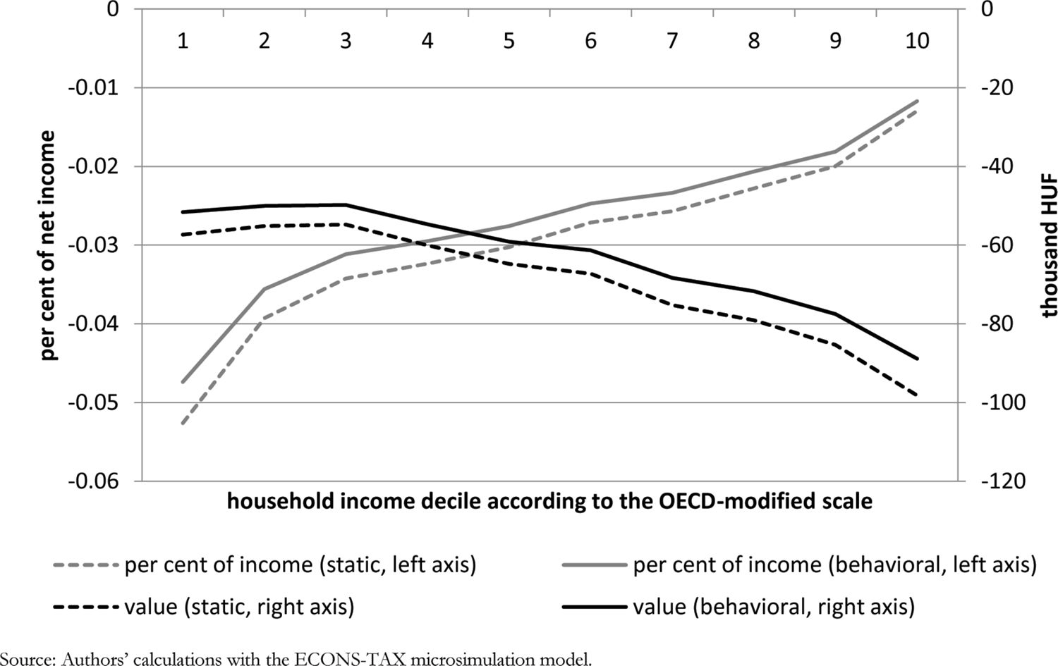
Change in VAT payments as a result of food VAT reduction by household income decile (decile 1 with the lowest income).
Source: Authors’ calculations with the ECONS-TAX microsimulation model.
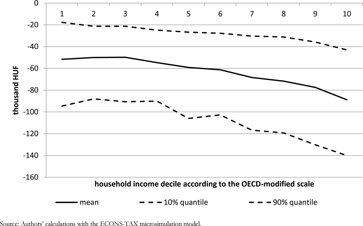
Mean and 10% and 90% quantiles of the change in VAT payments by household income decile (decile 1 with the lowest income).
Source: Authors’ calculations with the ECONS-TAX microsimulation model.
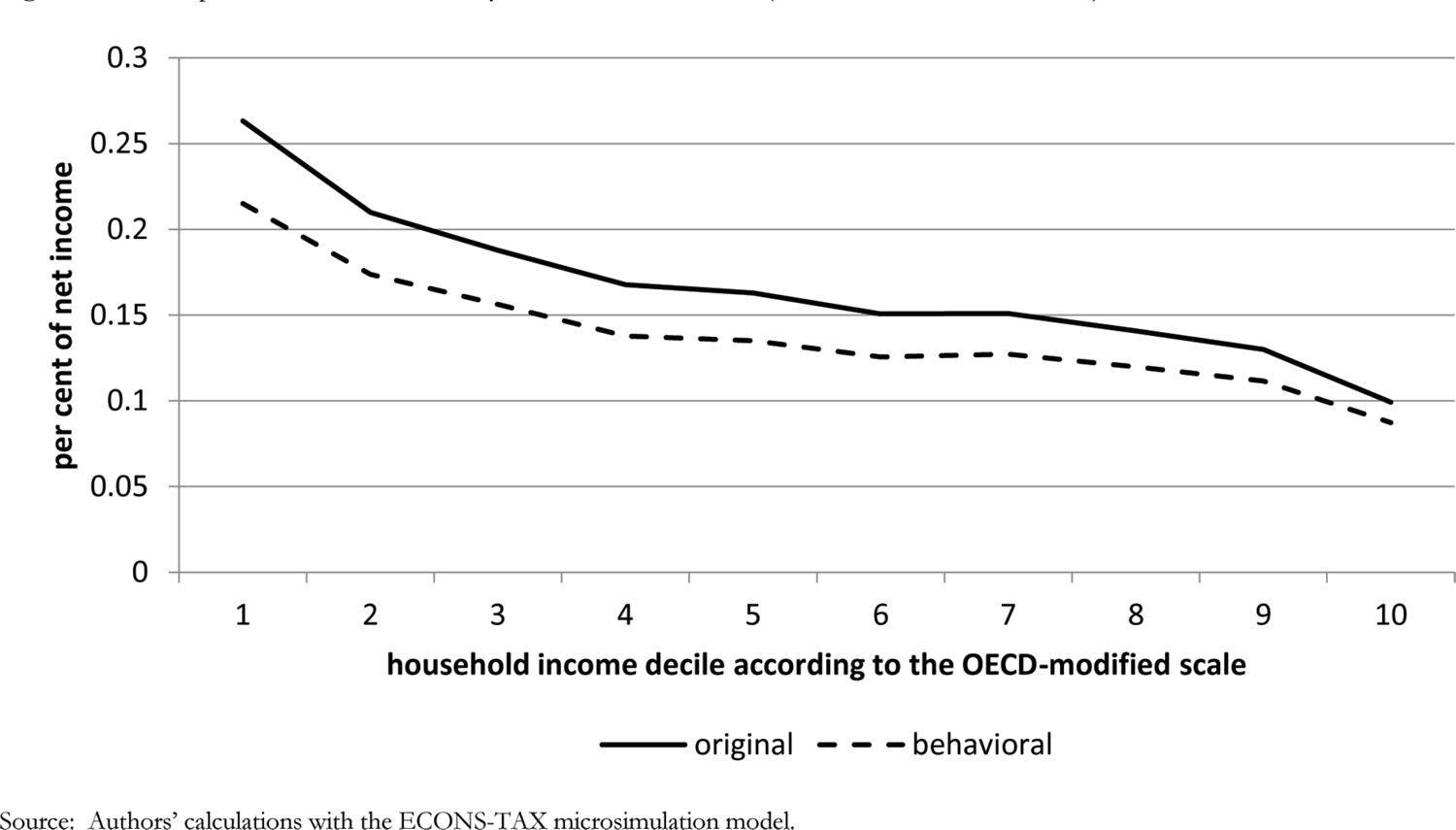
Pre- and post-reform VAT burdens by household income decile (decile 1 with the lowest income).
Source: Authors’ calculations with the ECONS-TAX microsimulation model.
5.3 Robustness check
Table 4 reports the results of the robustness checks with various country-level constant values for the Frisch-parameter. Six scenarios are covered in the table including the non-behavioural scenario. The variations in the results between different parameter assumptions seem to be limited. If demand for food is assumed to be relatively inelastic to price, then there is a smaller change in food consumption as a result of the VAT change and thus the decrease in VAT payment is slightly smaller. The table also shows that results from all behavioural scenarios are substantially different from the static scenario because the latter assumes no change in real consumption.
Changes in VAT payment by decile using different country-level constant Frisch parameters.
| Static scenario | Behavioural scenarios | |||||
|---|---|---|---|---|---|---|
| −1/ξ | 0.25 | 0.4 | 0.5 | 0.6 | 0.75 | |
| ξ | −4.0 | −2.5 | −2.0 | −1.67 | −1.33 | |
| Food price elasticity | −0.32 | −0.41 | −0.48 | −0.55 | −0.65 | |
| Income Decile | Change in VAT payment (thousand HUF) | |||||
| 1 | −57.3 | −50.3 | −51.1 | −51.6 | −52.2 | −53.0 |
| 2 | −55.1 | −48.8 | −49.5 | −50.0 | −50.5 | −51.2 |
| 3 | −54.8 | −48.6 | −49.3 | −49.8 | −50.3 | −51.0 |
| 4 | −60.0 | −53.5 | −54.2 | −54.7 | −55.2 | −56.0 |
| 5 | −64.8 | −57.8 | −58.6 | −59.1 | −59.6 | −60.5 |
| 6 | −67.3 | −59.9 | −60.7 | −61.3 | −61.8 | −62.7 |
| 7 | −75.2 | −66.8 | −67.7 | −68.4 | −69.0 | −70.0 |
| 8 | −79.1 | −70.0 | −71.0 | −71.7 | −72.4 | −73.4 |
| 9 | −85.3 | −75.7 | −76.7 | −77.5 | −78.2 | −79.3 |
| 10 | −98.2 | −86.7 | −88.0 | −88.8 | −89.7 | −91.0 |
| Total | −69.7 | −61.8 | −62.7 | −63.3 | −63.9 | −64.8 |
-
Source: Authors’ calculations with the ECONS-TAX microsimulation model.
Table 5 displays the results of the two additional scenarios, where the Frisch-parameter is a function of household income. The first column repeats the result of country-level constant ξ = −2 as a reference, while the second and third columns show the scenarios with income semi-elasticities of 0.10 and 0.20, respectively. Neither of the household-specific scenarios modifies the distributional effects of the VAT change considerably. This result is due to the fact that the bulk of the effect comes from the static change, and the variation in price elasticity is not very large in the household-specific scenarios (although still consistent with the literature, see above).
Changes in VAT payment by decile using different household-specific Frisch parameters.
| Average value of −1/ξ | 0.5 | 0.5 | 0.5 |
| Income semi-elasticity of −1/ξ | 0.00 | 0.10 | 0.20 |
| Average food price elasticity | −0.48 | −0.48 | −0.48 |
| 5% quantile of food price elasticity | −0.48 | −0.54 | −0.61 |
| 95% quantile of food price elasticity | −0.48 | −0.42 | −0.36 |
| Income Decile | Change in VAT payment (thousand HUF) | ||
| 1 | −51.6 | −52.0 | −51.7 |
| 2 | −50.0 | −49.8 | −49.6 |
| 3 | −49.8 | −49.7 | −49.5 |
| 4 | −54.7 | −54.7 | −54.6 |
| 5 | −59.1 | −59.1 | −59.1 |
| 6 | −61.3 | −61.4 | −61.4 |
| 7 | −68.4 | −68.5 | −68.7 |
| 8 | −71.7 | −72.0 | −72.3 |
| 9 | −77.5 | −77.9 | −78.4 |
| 10 | −88.8 | −89.9 | −90.9 |
| Total | −63.3 | −63.5 | −63.6 |
-
Source: Authors’ calculations with the ECONS-TAX microsimulation.
It should be noted that the model does not consider the broader general equilibrium effect that may take place should the VAT reform be implemented. It is possible that the changes in real consumption would affect the labour supply, savings and production of the consumption products, although the spillover effects might be limited. The exclusion of saving behaviours might lead to a slightly overestimated result in the medium and higher income groups due to their higher marginal propensity to save. Similarly, our model does not consider changes in the labour market although the tax reduction may potentially alter labour supply as well as labour demand. However, such effects are likely to be small given the relatively small size of the budgetary change and the relatively large import/export sectors in Hungary. We also assume full collection of taxes, as we do not have further information on possible tax avoidance. Overall, our analysis indicates that the general direction of the distributional welfare effect of the reform is robust, even with substantial deviation from the baseline parameter assumptions. Behavioural adjustment in consumption as shown in our analysis is limited compared with the direct static effect where the consumption pattern has no change. This is also the case for similar studies (see, for example, Alm & El-Ganainy, 2013).
6. Conclusions
VAT reform is one of the key economic policy debates in Hungary. The present level of VAT is 27% in Hungary, which is the highest in the EU. Different industry interest groups make much effort to obtain a reduced VAT for their goods and services, since they believe that this may improve their relative (domestic) competitiveness. Although this assumption that lower VAT improves competitiveness is not always accepted (see, for example, Feldstein & Krugman, 1990), a lower VAT is nevertheless preferred by some producers (e.g. the meat trade in Hungary has lobbied for many years to reduce its specific VAT). Any change to VAT will likely alter the balance of the fiscal budget and the commodity consumption patterns in the country, and this would affect people differently at different segments of the income spectrum.
This paper examines the effects of food VAT reduction on the consumption structure using a behavioural model based on ECONS-TAX. Our simulation suggests that a reduction of 18% in the VAT for tier 1 food items and 22% for tier 2 food items will decrease the total VAT payable by 2.2% on average for all households taking into account the behavioural responses. These proposed VAT reductions would benefit higher income households more in absolute terms, but our results also suggest substantial reduction for lower income households as a proportion of their total income. The behavioural model in the simulation allows for a shift in the consumption structure due to changes in the relative prices. The simulation also suggests that an adoption of lower food VAT rates would likely cut total tax revenues even if consumption increased in the other product categories.
It should also be noted that our computations were based on the cross-sectional data available in the Hungarian version of the EU-SILC database. For the estimates of consumption, we used the Stone-Geary utility function and an exogenously determined Frisch-parameter — the elasticity of the marginal utility of expenditure, which was calibrated from previous country-level studies. Our robustness test suggests that the general direction and findings remain robust even with relatively large variations in the elasticities: changing the reciprocal of the country-level Frisch parameter by ±50% or allowing reasonable household-level variation in the parameter do not result in huge changes in VAT payments. Further research may consider using a longitudinal dataset where the price variations over time can be exploited, which may further improve the reliability of the simulation.
Footnotes
1.
2.
We note that there are certain producers with VAT exempt status on the one hand, and there are certain goods and services that are free from VAT on the other hand.
3.
For another behavioural microsimulation model in Hungary, which analyses labour supply responses to tax and benefit changes (see Benczúr et al., 2012).
4.
In the following microeconomic derivations we do not distinguish between income and expenditure because we assume that the saving rate is constant.
5.
There appears to be a typographical error in the estimated equation of Lahiri et al. (2000): if the OLS regression is reproduced on their data the constant term should be negative, with the same absolute value as in the paper.
6.
If the estimated price elasticities are strictly used to calculate consumption patterns in the simulated scenario, total consumption (as aggregated from the consumption of the product categories) would increase by a negligible 0.3%. However, the saving rate is mainly determined by macroeconomic factors not explicitly modelled here, hence we display the results by assuming that total consumption is constant. (This means a 0.3% change in the results.)
7.
the OECD-modified scale assigns a value of 1 to the household head, of 0.5 to each additional adult member and of 0.3 to each child aged under 14 years (see, for example, OECD, 2013: Framework for statistics on the distribution of household income, consumption and wealth, Ch. 8, Framework for integrated analysis, p. 173). Households are then grouped into income deciles according to their equivalent household income calculated as a ratio of net household income and the modified household size.
Appendix
A. Structure of the ECONS-TAX microsimulation model
ECOS-TAX is a static microsimulation model that simulates the net disposable income distribution of the Hungarian households based on the assumed macroeconomic developments and the personal income tax regime. It is based on the household budget survey. These data are adjusted by input alignment. Dynamic ageing is applied. ECOS-TAX has been used several times for the impact assessment of tax changes in Hungary (see details in Cserháti et al., 2012).
ECONS-TAX is a dynamic extension of the ECOS-TAX model. Three new modules have been developed to model the consumption, the labour supply and demand. Furthermore it is connected with a macroeconomic model consisting of a CGE and a monetary module. ECONS-TAX follows a TD-BU (top-down - bottom-up) approach, so it is possible to analyse both micro- and macro-level shocks and also the spillover effects.
During simulation, the dynamic labour market module obtains the industry-level wage and price indices as well as the industry- and cohort-specific employment rates as inputs. They may come from a macroeconomic model, from expert assessment or factual data corresponding to later years. The dynamic labour market module provides the employment status and gross income at the individual level as outputs, and gross income is then taxed by the static module according to the PIT and social contribution rules for the given year. In the dynamic labour market module, only unemployment benefits are simulated in a dynamic way among the social transfers.

Dynamic labour market module.
Source: Own construction.
B. Detailed results of the parameter estimations
Parameter estimates of the expenditure share equations.
| Share of product category | Av. of variable | Food and non-alc. beverages | Alcoholic beverages | Tobacco | Clothing and footwear | Water and energy | Rents | Household services | Health |
|---|---|---|---|---|---|---|---|---|---|
| Log expenditure | 14.3 | 0.300*** | −0.0152 | −0.0287 | 0.0562* | −0.255*** | 0.101*** | 0.153*** | 0.0996*** |
| (0.536) | (0.0519) | (0.0135) | (0.0236) | (0.0297) | (0.0536) | (0.0188) | (0.0338) | (0.0342) | |
| Log expenditure squared | 206.0 | −0.0119*** | 0.000552 | 0.000701 | −0.00150 | 0.00513*** | −0.00318*** | −0.00589*** | −0.00340*** |
| (15.4) | (0.00178) | (0.000459) | (0.000803) | (0.00104) | (0.00184) | (0.000640) | (0.00116) | (0.00117) | |
| Household type (baseline = no retired person, no couple, no child in the household) (average = 0.179, standard deviation = 0.383 for baseline variable) | |||||||||
| Retired: no; couple: no; child: yes | 0.032 | 0.0132** | −0.00457*** | −0.00422** | 0.00959*** | 0.0167*** | −0.00896** | 0.00197 | −0.00683*** |
| (0.176) | (0.00603) | (0.000761) | (0.00204) | (0.00283) | (0.00464) | (0.00386) | (0.00364) | (0.00239) | |
| Retired: no; couple: yes; child: no | 0.201 | 0.0338*** | −0.00107 | −1.58e-05 | −0.00124 | 0.0210*** | −0.00662*** | −0.00494*** | 0.00865*** |
| (0.401) | (0.00311) | (0.000731) | (0.00141) | (0.00145) | (0.00245) | (0.00208) | (0.00184) | (0.00156) | |
| Retired: no; couple: yes; child: yes | 0.172 | 0.0198*** | −0.00383*** | −0.00205 | 0.00466* | 0.0261*** | −0.0128*** | −0.00305 | 0.00972*** |
| (0.377) | (0.00509) | (0.000867) | (0.00196) | (0.00243) | (0.00356) | (0.00312) | (0.00263) | (0.00203) | |
| Retired: yes; couple: no; child: no | 0.210 | −0.00967** | −0.00137 | −0.00111 | −0.00346* | 0.00610 | −0.00950*** | −0.00183 | 0.00970*** |
| (0.408) | (0.00461) | (0.000984) | (0.00157) | (0.00179) | (0.00380) | (0.00203) | (0.00298) | (0.00323) | |
| Retired: yes; couple: no; child: yes | 0.00458 | 0.0317** | −0.00624*** | −0.00652 | −0.000390 | 0.0282*** | −0.0159*** | 0.00924 | 0.0269*** |
| (0.0675) | (0.0136) | (0.00157) | (0.00426) | (0.00516) | (0.0105) | (0.00531) | (0.00994) | (0.00670) | |
| Retired: yes; couple: yes; child: no | 0.181 | 0.0159*** | −0.000923 | 0.00106 | −0.00380 | 0.0248*** | −0.0136*** | −0.0116*** | 0.0191*** |
| (0.385) | (0.00609) | (0.00138) | (0.00218) | (0.00269) | (0.00482) | (0.00226) | (0.00373) | (0.00408) | |
| Retired: yes; couple: yes; child: yes | 0.0204 | 0.0111 | −0.00433*** | −0.00115 | −0.000883 | 0.0395*** | −0.0134*** | −0.0132*** | 0.0264*** |
| (0.141) | (0.00817) | (0.00144) | (0.00300) | (0.00376) | (0.00608) | (0.00373) | (0.00458) | (0.00472) | |
| Number of children (0-15 years) | 0.370 | 0.0227*** | −0.000507 | −0.000336 | −0.000577 | 0.00377** | −0.00302** | −0.000199 | −0.00215*** |
| (0.785) | (0.00241) | (0.000315) | (0.000905) | (0.00110) | (0.00154) | (0.00134) | (0.00116) | (0.000810) | |
| Number of retired people | 0.536 | 0.0118*** | 0.000843 | −0.000554 | 0.000522 | 0.00372 | −0.00103 | 0.00754*** | −0.00186 |
| (0.703) | (0.00358) | (0.000794) | (0.00111) | (0.00148) | (0.00277) | (0.00102) | (0.00223) | (0.00251) | |
| Number of earners | 0.938 | 0.000274 | −0.000421* | −0.00128** | 0.00492*** | 0.00700*** | −0.00268*** | 0.000789 | −0.00824*** |
| (0.949) | (0.00136) | (0.000231) | (0.000553) | (0.000605) | (0.00101) | (0.000608) | (0.000731) | (0.000676) | |
| Cigarette smoker in the household | 0.379 | −0.00727*** | 0.00273*** | 0.0594*** | −0.00315*** | −0.00654*** | 0.00252** | −0.00477*** | −0.00592*** |
| (0.485) | (0.00177) | (0.000382) | (0.000786) | (0.000805) | (0.00142) | (0.000987) | (0.00108) | (0.00103) | |
| Car in the household | 0.461 | −0.0335*** | −0.000903** | −0.00437*** | −0.00244*** | 0.000899 | −0.0130*** | −0.0136*** | −0.00825*** |
| (0.498) | (0.00202) | (0.000389) | (0.000705) | (0.000928) | (0.00153) | (0.00114) | (0.00122) | (0.00116) | |
| Household head | |||||||||
| Female | 0.472 | −0.00450** | −0.00449*** | −0.00244*** | −0.00542*** | 0.00663*** | −0.00212** | 0.00607*** | 0.00591*** |
| (0.499) | (0.00190) | (0.000445) | (0.000768) | (0.000893) | (0.00151) | (0.00107) | (0.00115) | (0.00111) | |
| Standardised age (in 10 years) (standardized to 50 years) | 0.483 | 0.00730*** | 0.000656** | −0.000905 | −0.00515*** | 0.00844*** | −0.00389*** | 0.00295*** | 0.00816*** |
| (1.45) | (0.00173) | (0.000330) | (0.000671) | (0.000747) | (0.00134) | (0.00107) | (0.000977) | (0.000889) | |
| Standardized age squared | 2.33 | −0.00308*** | −0.000185* | −0.000984*** | 0.000189 | −0.00269*** | 0.00369*** | 0.000274 | 0.00282*** |
| (2.50) | (0.000544) | (9.53e-05) | (0.000198) | (0.000253) | (0.000418) | (0.000465) | (0.000299) | (0.000278) | |
| Standardized age on the third power | 2.83 | −0.000518* | −0.000123** | 5.58e-05 | 2.76e-06 | −3.97e-05 | −0.000912*** | −0.000161 | 0.000943*** |
| (8.08) | (0.000298) | (5.28e-05) | (0.000104) | (0.000127) | (0.000232) | (0.000219) | (0.000168) | (0.000165) | |
| Level of education of household head (baseline = never attended school) (average = 0.00099, standard deviation = 0.0315 for baseline variable) | |||||||||
| Less than 8 classes in primary school | 0.0392 | −0.0711 | 0.00135 | −0.00153 | 0.00735* | 0.0719*** | −0.0248 | 0.0320* | −0.0280 |
| (0.194) | (0.0466) | (0.00401) | (0.0150) | (0.00400) | (0.0264) | (0.0192) | (0.0169) | (0.0266) | |
| 8 to 10 years of primary school | 0.198 | −0.0864* | −7.37e-05 | −0.00123 | 0.00388 | 0.0680*** | −0.0253 | 0.0395** | −0.0216 |
| (0.399) | (0.0463) | (0.00392) | (0.0150) | (0.00371) | (0.0261) | (0.0191) | (0.0166) | (0.0263) | |
| Lower secondary education | 0.321 | −0.110** | 0.000610 | −0.00363 | 0.000977 | 0.0688*** | −0.0238 | 0.0520*** | −0.0220 |
| (0.467) | (0.0462) | (0.00392) | (0.0150) | (0.00370) | (0.0261) | (0.0191) | (0.0166) | (0.0263) | |
| Secondary education | 0.133 | −0.115** | 0.00114 | −0.00468 | 0.00356 | 0.0597** | −0.0251 | 0.0569*** | −0.0282 |
| (0.340) | (0.0463) | (0.00393) | (0.0150) | (0.00377) | (0.0261) | (0.0191) | (0.0167) | (0.0263) | |
| Upper secondary education | 0.0778 | −0.118** | 0.000149 | −0.00606 | 0.00106 | 0.0598** | −0.0210 | 0.0524*** | −0.0281 |
| (0.268) | (0.0463) | (0.00394) | (0.0150) | (0.00384) | (0.0262) | (0.0192) | (0.0167) | (0.0264) | |
| Post-secondary non-tertiary education | 0.0408 | −0.117** | 0.00307 | −0.00555 | −0.00266 | 0.0501* | −0.0217 | 0.0549*** | −0.0215 |
| (0.198) | (0.0464) | (0.00399) | (0.0150) | (0.00399) | (0.0262) | (0.0193) | (0.0168) | (0.0265) | |
| Adult school | 0.0122 | −0.124*** | −0.000219 | −0.00888 | 0.00762 | 0.0564** | −0.0294 | 0.0619*** | −0.0222 |
| (0.110) | (0.0466) | (0.00404) | (0.0151) | (0.00544) | (0.0266) | (0.0194) | (0.0173) | (0.0266) | |
| College | 0.101 | −0.124*** | 0.00160 | −0.00502 | 0.00719* | 0.0535** | −0.0238 | 0.0542*** | −0.0245 |
| (0.301) | (0.0463) | (0.00396) | (0.0150) | (0.00388) | (0.0261) | (0.0192) | (0.0167) | (0.0264) | |
| University | 0.0713 | −0.128*** | 0.00187 | −0.00331 | 0.0136*** | 0.0489* | −0.0252 | 0.0542*** | −0.0235 |
| (0.257) | (0.0463) | (0.00396) | (0.0150) | (0.00410) | (0.0261) | (0.0192) | (0.0167) | (0.0264) | |
| PhD | 0.00448 | −0.127*** | 0.000706 | −0.00288 | 0.0154** | 0.0441 | −0.0321* | 0.0547*** | −0.0410 |
| (0.0668) | (0.0472) | (0.00446) | (0.0157) | (0.00752) | (0.0271) | (0.0195) | (0.0177) | (0.0269) | |
| Constant | −1.516*** | 0.116 | 0.280 | −0.457** | 2.714*** | −0.739*** | −0.923*** | −0.659*** | |
| (0.382) | (0.0985) | (0.173) | (0.212) | (0.391) | (0.139) | (0.247) | (0.251) | ||
| Number of observations | 10,041 | 10,041 | 10,041 | 10,041 | 10,041 | 10,041 | 10,041 | 10,041 | |
| R-squared | 0.200 | 0.040 | 0.505 | 0.188 | 0.428 | 0.088 | 0.108 | 0.299 | |
| Share of product category | Private transport | Public transport | Communication | Recreation and culture | Education | Restaurants and hotels | Other | Durable goods |
|---|---|---|---|---|---|---|---|---|
| Log expenditure | 0.205*** | 0.160*** | 0.248*** | 0.0933*** | −0.00532 | 0.0290 | −1.174*** | 0.0336 |
| (0.0287) | (0.0172) | (0.0291) | (0.0325) | (0.0127) | (0.0479) | (0.134) | (0.0974) | |
| Log expenditure squared | −0.00703*** | −0.00534*** | −0.00906*** | −0.00268** | 0.000331 | −7.86e-05 | 0.0423*** | 0.00102 |
| (0.00101) | (0.000590) | (0.00101) | (0.00114) | (0.000450) | (0.00168) | (0.00475) | (0.00343) | |
| Household type (baseline = no retired person, no couple, no child in the household) | ||||||||
| Retired: no; couple: no; child: yes | −0.00637** | −0.00250 | 0.00568** | 0.00121 | 0.00264* | −0.0120*** | 0.00367 | −0.00914 |
| (0.00293) | (0.00232) | (0.00278) | (0.00260) | (0.00135) | (0.00363) | (0.00489) | (0.00573) | |
| Retired: no; couple: yes; child: no | −0.00254 | −0.00435*** | 0.00140 | −0.00566*** | 0.00113 | −0.0206*** | −0.00556** | −0.0135*** |
| (0.00178) | (0.00134) | (0.00131) | (0.00145) | (0.000893) | (0.00196) | (0.00234) | (0.00309) | |
| Retired: no; couple: yes; child: yes | −0.00556** | −0.00637*** | 0.00308 | −0.00733*** | −0.000267 | −0.0214*** | 0.00179 | −0.00253 |
| (0.00279) | (0.00191) | (0.00210) | (0.00218) | (0.00105) | (0.00274) | (0.00394) | (0.00486) | |
| Retired: yes; couple: no; child: no | 0.00377 | −0.00564*** | 0.00249 | 6.94e-06 | −0.00136 | −0.00132 | 0.00869** | 0.00450 |
| (0.00248) | (0.00154) | (0.00187) | (0.00205) | (0.000961) | (0.00276) | (0.00362) | (0.00473) | |
| Retired: yes; couple: no; child: yes | −0.00566 | 1.02e-05 | −0.00100 | −0.00969** | −0.00150 | −0.0207*** | −0.0151*** | −0.0133 |
| (0.00577) | (0.00589) | (0.00484) | (0.00442) | (0.00151) | (0.00482) | (0.00572) | (0.0116) | |
| Retired: yes; couple: yes; child: no | 0.00645* | −0.00342* | 0.00627** | −0.00929*** | −0.000900 | −0.0170*** | 0.00479 | −0.0179*** |
| (0.00371) | (0.00203) | (0.00259) | (0.00275) | (0.00136) | (0.00356) | (0.00487) | (0.00639) | |
| Retired: yes; couple: yes; child: yes | −0.000977 | −0.00413 | 0.00787** | −0.0109*** | −0.000602 | −0.0222*** | −0.00128 | −0.0118 |
| (0.00488) | (0.00279) | (0.00323) | (0.00346) | (0.00135) | (0.00399) | (0.00630) | (0.00805) | |
| Number of children (0-15 years) | −0.00125 | −0.00240*** | −0.00422*** | 9.84e-05 | 0.000503 | −0.00241** | −0.00312* | −0.00692*** |
| (0.00119) | (0.000718) | (0.000882) | (0.000831) | (0.000407) | (0.000985) | (0.00165) | (0.00210) | |
| Number of retired people | −0.00486** | −0.00183* | −0.000995 | 0.00297* | −0.000876 | −0.00692*** | −0.00490* | −0.00358 |
| (0.00206) | (0.000972) | (0.00143) | (0.00158) | (0.000622) | (0.00187) | (0.00265) | (0.00364) | |
| Number of earners | 0.00131* | 0.00497*** | 0.00656*** | 0.000945* | 0.000467 | 0.00248*** | −0.00628*** | −0.0108*** |
| (0.000758) | (0.000539) | (0.000554) | (0.000551) | (0.000347) | (0.000722) | (0.00117) | (0.00135) | |
| Cigarette smoker in the household | −0.00381*** | −0.00174** | −0.00223*** | −0.00738*** | −0.000259 | −0.00743*** | −0.00777*** | −0.00634*** |
| (0.000996) | (0.000689) | (0.000744) | (0.000811) | (0.000432) | (0.00108) | (0.00141) | (0.00181) | |
| Car in the household | 0.0973*** | −0.0140*** | 0.00187** | −0.00558*** | −0.000587 | −0.0104*** | 0.00432** | 0.00225 |
| (0.00128) | (0.000807) | (0.000826) | (0.000954) | (0.000460) | (0.00122) | (0.00170) | (0.00193) | |
| Household head | ||||||||
| Female | −0.00601*** | 0.00161** | 0.00184** | −0.000424 | 0.00152*** | −0.00348*** | 0.00418*** | 0.00111 |
| (0.00110) | (0.000715) | (0.000789) | (0.000893) | (0.000483) | (0.00123) | (0.00149) | (0.00197) | |
| Standardised age (in 10 years) | −0.000454 | −0.000943 | −0.00218*** | −0.00385*** | −0.00106*** | −0.00693*** | −0.00159 | −0.000551 |
| (0.000947) | (0.000693) | (0.000719) | (0.000827) | (0.000393) | (0.00108) | (0.00126) | (0.00170) | |
| Standardized age squared | −0.000257 | −0.000864*** | −0.00118*** | 0.000533** | −0.000415*** | 0.00234*** | −0.000342 | 0.000142 |
| (0.000277) | (0.000215) | (0.000215) | (0.000258) | (0.000148) | (0.000341) | (0.000380) | (0.000497) | |
| Standardized age on the third power | −8.22e-05 | −0.000176 | 0.000289** | 9.84e-05 | 0.000122* | 0.000427** | 4.33e-05 | 2.95e-05 |
| (0.000150) | (0.000109) | (0.000115) | (0.000135) | (7.10e-05) | (0.000180) | (0.000208) | (0.000272) | |
| Level of education of household head (baseline = never attended school) | ||||||||
| Less than 8 classes in primary school | −0.0160 | 0.00407 | 0.0196* | −0.000814 | 0.000465 | 0.00227 | 0.00660 | −0.00341 |
| (0.0147) | (0.00431) | (0.0115) | (0.00621) | (0.00155) | (0.00401) | (0.0239) | (0.0143) | |
| 8 to 10 years of primary school | −0.0198 | 0.00253 | 0.0226** | 0.00440 | −2.15e-05 | 0.00453 | 0.00399 | 0.00492 |
| (0.0146) | (0.00425) | (0.0114) | (0.00605) | (0.00155) | (0.00328) | (0.0237) | (0.0137) | |
| Lower secondary education | −0.0171 | 0.00393 | 0.0315*** | 0.00978 | −0.000305 | 0.00866*** | 0.00651 | −0.00581 |
| (0.0147) | (0.00426) | (0.0114) | (0.00606) | (0.00157) | (0.00334) | (0.0237) | (0.0137) | |
| Secondary education | −0.0174 | 0.00800* | 0.0362*** | 0.0188*** | 0.000708 | 0.0157*** | 0.00475 | −0.0148 |
| (0.0147) | (0.00432) | (0.0114) | (0.00614) | (0.00164) | (0.00355) | (0.0238) | (0.0138) | |
| Upper secondary education | −0.0196 | 0.00689 | 0.0387*** | 0.0217*** | 0.00283 | 0.0171*** | 0.00464 | −0.0129 |
| (0.0147) | (0.00439) | (0.0115) | (0.00622) | (0.00175) | (0.00375) | (0.0238) | (0.0140) | |
| Post-secondary non-tertiary education | −0.0195 | 0.00688 | 0.0366*** | 0.0204*** | −0.000173 | 0.0174*** | 0.00389 | −0.00555 |
| (0.0149) | (0.00446) | (0.0115) | (0.00641) | (0.00179) | (0.00431) | (0.0239) | (0.0143) | |
| Adult school | −0.0136 | 0.00769 | 0.0406*** | 0.0228*** | 0.00171 | 0.0148** | −0.000832 | −0.0146 |
| (0.0152) | (0.00500) | (0.0118) | (0.00721) | (0.00258) | (0.00596) | (0.0243) | (0.0155) | |
| College | −0.0171 | 0.00703 | 0.0384*** | 0.0286*** | 0.00160 | 0.0214*** | 0.000975 | −0.0199 |
| (0.0147) | (0.00437) | (0.0114) | (0.00624) | (0.00180) | (0.00375) | (0.0238) | (0.0139) | |
| University | −0.0179 | 0.00932** | 0.0401*** | 0.0453*** | 0.00153 | 0.0265*** | −0.0119 | −0.0320** |
| (0.0148) | (0.00442) | (0.0115) | (0.00648) | (0.00183) | (0.00422) | (0.0240) | (0.0141) | |
| PhD | −0.00759 | 0.0141* | 0.0399*** | 0.0438*** | −0.00240 | 0.0423*** | −0.00610 | −0.0357* |
| (0.0169) | (0.00737) | (0.0123) | (0.0100) | (0.00265) | (0.00957) | (0.0268) | (0.0184) | |
| Constant | −1.455*** | −1.172*** | −1.668*** | −0.747*** | 0.0141 | −0.362 | 8.177*** | −0.602 |
| (0.203) | (0.125) | (0.210) | (0.231) | (0.0901) | (0.341) | (0.946) | (0.692) | |
| Number of observations | 10,041 | 10,041 | 10,041 | 10,041 | 10,041 | 10,041 | 10,041 | 10,041 |
| R-squared | 0.572 | 0.116 | 0.094 | 0.182 | 0.051 | 0.144 | 0.166 | 0.086 |
-
Source: Authors’ calculations based on HKÉF 2011. Heteroscedasticity-robust standard errors are displayed in parentheses.
-
(*)
Significance levels: 10%
-
(**)
Significance levels: 5%
-
(***)
Significance levels: 1%
Expenditure elasticities by household type.
| Household type | Total | ||||||||
|---|---|---|---|---|---|---|---|---|---|
| Retired | no | no | no | no | yes | yes | yes | yes | |
| Couple | no | no | yes | yes | no | no | yes | yes | |
| Child | no | yes | no | yes | no | yes | no | yes | |
| Food and non-alc. beverages | 0.77 | 0.82 | 0.74 | 0.75 | 0.82 | 0.83 | 0.77 | 0.74 | 0.77 |
| Alcoholic beverages | 1.06 | 1.17 | 1.09 | 1.17 | 1.06 | 1.30 | 1.08 | 1.16 | 1.09 |
| Tobacco | 0.65 | 0.62 | 0.63 | 0.60 | 0.47 | 0.75 | 0.54 | 0.71 | 0.58 |
| Clothing and footwear | 1.27 | 1.24 | 1.22 | 1.19 | 1.56 | 1.28 | 1.32 | 1.22 | 1.31 |
| Water and energy | 0.35 | 0.41 | 0.34 | 0.31 | 0.45 | 0.44 | 0.39 | 0.38 | 0.37 |
| Rents | 1.29 | 1.56 | 1.56 | 1.75 | 1.80 | 1.55 | 1.80 | 1.80 | 1.64 |
| Household services | 0.83 | 0.84 | 0.74 | 0.73 | 0.87 | 0.85 | 0.78 | 0.71 | 0.79 |
| Health | 1.07 | 1.10 | 0.98 | 0.98 | 1.04 | 1.02 | 1.00 | 0.96 | 1.02 |
| Private transport | 1.07 | 1.08 | 0.98 | 0.97 | 1.21 | 1.06 | 0.99 | 0.95 | 1.05 |
| Public transport | 1.30 | 1.30 | 1.12 | 1.15 | 1.80 | 1.28 | 1.36 | 1.07 | 1.35 |
| Communications | 0.84 | 0.83 | 0.75 | 0.69 | 0.86 | 0.79 | 0.74 | 0.67 | 0.78 |
| Recreation and culture | 1.25 | 1.27 | 1.25 | 1.25 | 1.43 | 1.32 | 1.30 | 1.33 | 1.30 |
| Education | 1.47 | 1.30 | 1.44 | 1.43 | 1.80 | 1.80 | 1.80 | 1.64 | 1.59 |
| Restaurants and hotels | 1.51 | 1.59 | 1.67 | 1.66 | 1.80 | 1.80 | 1.80 | 1.80 | 1.69 |
| Other goods and services | 1.61 | 1.66 | 1.80 | 1.80 | 1.19 | 1.80 | 1.68 | 1.80 | 1.61 |
| Durable goods | 1.80 | 1.80 | 1.80 | 1.75 | 1.80 | 1.80 | 1.80 | 1.80 | 1.79 |
-
Source: Authors’ calculations based on HKÉF for year 2011.
Price elasticities by household type.
| Household type | Total | ||||||||
|---|---|---|---|---|---|---|---|---|---|
| Retired | no | no | no | no | yes | yes | yes | yes | |
| Couple | no | no | yes | yes | no | no | yes | yes | |
| Child | no | yes | no | yes | no | yes | no | yes | |
| Food and non-alc. beverages | −0.47 | −0.52 | −0.46 | −0.47 | −0.51 | −0.54 | −0.48 | −0.46 | −0.48 |
| Alcoholic beverages | −0.53 | −0.59 | −0.55 | −0.59 | −0.53 | −0.65 | −0.55 | −0.58 | −0.55 |
| Tobacco | −0.34 | −0.32 | −0.32 | −0.31 | −0.24 | −0.39 | −0.28 | −0.37 | −0.30 |
| Clothing and footwear | −0.66 | −0.65 | −0.63 | −0.63 | −0.79 | −0.66 | −0.68 | −0.64 | −0.68 |
| Water and energy | −0.22 | −0.26 | −0.21 | −0.19 | −0.30 | −0.28 | −0.25 | −0.24 | −0.24 |
| Rents | −0.66 | −0.79 | −0.78 | −0.88 | −0.90 | −0.78 | −0.90 | −0.90 | −0.83 |
| Household services | −0.46 | −0.47 | −0.41 | −0.40 | −0.48 | −0.48 | −0.43 | −0.39 | −0.44 |
| Health | −0.55 | −0.56 | −0.51 | −0.50 | −0.56 | −0.54 | −0.54 | −0.50 | −0.53 |
| Private transport | −0.56 | −0.56 | −0.53 | −0.53 | −0.62 | −0.55 | −0.54 | −0.52 | −0.56 |
| Public transport | −0.66 | −0.66 | −0.57 | −0.58 | −0.90 | −0.65 | −0.68 | −0.54 | −0.68 |
| Communications | −0.46 | −0.45 | −0.41 | −0.38 | −0.46 | −0.43 | −0.40 | −0.37 | −0.42 |
| Recreation and culture | −0.66 | −0.66 | −0.65 | −0.65 | −0.73 | −0.68 | −0.67 | −0.68 | −0.67 |
| Education | −0.74 | −0.66 | −0.73 | −0.72 | −0.90 | −0.90 | −0.90 | −0.82 | −0.80 |
| Restaurants and hotels | −0.77 | −0.81 | −0.85 | −0.84 | −0.91 | −0.90 | −0.90 | −0.90 | −0.86 |
| Other goods and services | −0.82 | −0.85 | −0.91 | −0.92 | −0.65 | −0.91 | −0.87 | −0.92 | −0.83 |
| Durable goods | −0.91 | −0.91 | −0.91 | −0.89 | −0.91 | −0.91 | −0.91 | −0.91 | −0.91 |
-
Source: Authors’ calculations based on HKÉF for year 2011.
Changes in VAT payments by household income decile and household type (thousand HUF).
| Income decile | Household type | Total | ||||||||
|---|---|---|---|---|---|---|---|---|---|---|
| Retired | no | no | no | no | yes | yes | yes | yes | ||
| Couple | no | no | yes | yes | no | no | yes | yes | ||
| Child | no | yes | no | yes | no | yes | no | yes | ||
| 1 | −32.7 | −56.8 | −53.9 | −73.5 | −31.1 | −69.7 | −60.7 | −77.1 | −51.6 | |
| 2 | −35.9 | −56.3 | −59.4 | −66.4 | −38.7 | −43.4 | −55.9 | −61.9 | −50.0 | |
| 3 | −47.7 | −51.0 | −58.5 | −69.8 | −37.3 | −76.2 | −50.2 | −91.6 | −49.8 | |
| 4 | −46.6 | −55.9 | −65.6 | −76.1 | −40.0 | −77.5 | −55.6 | −82.3 | −54.7 | |
| 5 | −46.8 | −62.4 | −64.5 | −73.2 | −46.7 | −60.0 | −65.0 | −65.4 | −59.1 | |
| 6 | −44.3 | −57.2 | −70.8 | −75.5 | −45.1 | −98.1 | −63.9 | −85.9 | −61.3 | |
| 7 | −54.2 | −54.6 | −73.8 | −79.3 | −51.5 | −77.1 | −70.5 | −93.4 | −68.4 | |
| 8 | −51.3 | −68.3 | −76.6 | −78.3 | −57.9 | −71.5 | −77.6 | −77.3 | −71.7 | |
| 9 | −50.5 | −83.5 | −82.1 | −85.9 | −59.1 | −73.7 | −83.3 | −119.8 | −77.5 | |
| 10 | −64.8 | −78.3 | −95.6 | −94.6 | −69.0 | −103.0 | −91.4 | −118.0 | −88.8 | |
| Total | −45.7 | −59.0 | −72.8 | −78.0 | −44.1 | −73.1 | −69.8 | −87.7 | −63.3 | |
-
Source: Authors’ calculations based on HKÉF for year 2011. Household income decile is defined according to the OECD-modified scale.
References
-
1
The distributional impact of reforms to direct and indirect tax in Mexico: Methodological Issues and ApproachInstitute for Fiscal Studies.
-
2
Value added taxation and consumptionInternational Tax and Public Finance 20:105–128.
-
3
The impact of food prices on consumption: A systematic review of research on the price elasticity of demand for foodAmerican Journal of Public Health 100:216–222.
-
4
Measuring consumer preferences and estimating demand systemsIn: D Slottje, editors. Quantifying Consumer Preferences, Contributions to Economic Analysis. Bingley: Emerald Press. pp. 1–35.
-
5
Quadratic Engel curves and consumer demandThe Review of Economics and Statistics 79:527–539.
-
6
Assessing changes of the Hungarian tax and transfer system, a general equilibrium microsimulation approach. MNB Working Papers, 2012/7Assessing changes of the Hungarian tax and transfer system, a general equilibrium microsimulation approach. MNB Working Papers, 2012/7.
-
7
Assessment of income distribution in Hungary using a microsimulation model (No. 10). Working PaperMinistry of Finance.
-
8
Mikroszimulációs elemzés a személyi jövedelemadó módosításainak hatásvizsgálatában. (Microsimulation analysis in the impact assessment of changes of personal income tax.)Közgazdasági Szemle (Economic Review – monthly of the Hungarian Academy of Sciences) 58:97–110.
-
9
Tax avoidance, tax evasion, black and grey employmentIn: K Fazekas, P Benczúr, Á Telegdy, editors. The Hungarian Labour Market, Review and Analysis 2013. Institute of Economics, Hungarian Academy of Sciences. pp. 161–184.
-
10
Welfare effects of tax reform: a general equilibrium analysisInternational Tax and Finance 19:368–392.
-
11
Handbook of microsimulation modellingConsumption and indirect tax models, Handbook of microsimulation modelling, Chapter 8, Emerald Group Publishing.
- 12
-
13
Measuring the welfare effects of price changes, a convenient parametric approach. Australian Economic Papers137–151, Measuring the welfare effects of price changes, a convenient parametric approach. Australian Economic Papers, 37, 2.
-
14
Háztartási fogyasztói magatartás és jólét Magyarországon a rendszerváltás után. (Household consumer behaviour and welfare in Hungary since the change of system.)Közgazdasági Szemle (Economic Review – monthly of the Hungarian Academy of Sciences) 55:107–135.
-
15
Pénzt vagy életet? Empirikus eredmények néhány gazdaságpolitikai beavatkozás heterogén jóléti hatásairól. (Money or life? Empirical results about the heterogenous welfare effects of some economic policy changes.)Közgazdasági Szemle (Economic Review – monthly of the Hungarian Academy of Sciences) 63:901–943.
-
16
Examination of income inequalities of Hungarian households in 2012 using a microsimulation modelHungarian Statistical Review 90:3–17.
-
17
Distributional impact analysis of the 2015 Hungarian national budget5th World Congress of the International Microsimulation Association 2-4 September 2015.
-
18
Flat rate tax in HungaryJournal of International Scientific Publication: Economy and Business 5:489–497.
-
19
The software prepared for the household statistics microsimulation in the Hungarian CSOPaper prepared for IIASA International Workshop on Demographic Microsimulation.
-
20
A Reconsideration of the Empirical Implications of Additive PreferencesThe Economic Journal 84:338–348.
- 21
-
22
How regressive are indirect taxes? A microsimulation analysis for five European countriesJournal of Policy Analysis and Management 29:326–350.
- 23
-
24
Integrating VAT in Euromod. (FLEMOSI Discussion Paper No. 32), April 2014Integrating VAT in Euromod. (FLEMOSI Discussion Paper No. 32), April 2014.
-
25
Macroeconomic effects of a shift from direct to indirect taxation: A simulation for 15 EU member states. Technical Report, European Commission services (DG TAXUD), 72nd meeting of the OECD Working Party No. 2 on Tax Policy Analysis and Tax Statistics, Paris, 14-16 November 2006Macroeconomic effects of a shift from direct to indirect taxation: A simulation for 15 EU member states. Technical Report, European Commission services (DG TAXUD), 72nd meeting of the OECD Working Party No. 2 on Tax Policy Analysis and Tax Statistics, Paris, 14-16 November 2006.
-
26
Taxation in the global economy, Section III.7263–282, International trade effects of value added taxation, Taxation in the global economy, Section III.7, University Chicago Press, ISBN 0-226-70591-9.
-
27
Handbook of Income Distribution2141–2221, Microsimulation and policy analysis, Handbook of Income Distribution.
-
28
A complete scheme for computing all direct and cross demand elasticities in a model with many sectorsEconometrica 27:177–196.
-
29
Does Indirect Tax Increase the Income Gap between Urban and Rural Areas?Open Journal of Social Sciences 4:170–176.
-
30
The effect of the change in VAT rates on the consumer price index. MNB Bulletin, December 200614–20, The effect of the change in VAT rates on the consumer price index. MNB Bulletin, December 2006.
- 31
-
32
Exemption versus zero rating: A hidden problem of VATJournal of Public Economics 46:307–328.
-
33
The effect of rising food prices on food consumption: systematic review with meta-regressionBMJ 346:f3703.
-
34
The redistributive potential of taxation in Latin America. CEPAL Review 116, August 2015The redistributive potential of taxation in Latin America. CEPAL Review 116, August 2015.
-
35
Macroeconomic Policies and Structural ReformCombatting unemployment: Is flexibility enough?, Macroeconomic Policies and Structural Reform, Paris, OECD.
-
36
The targeting of zero-rated basic foodstuffs under value added tax (VAT) in South AfricaJournal for Studies in Economics and Econometrics 37:87–104.
-
37
The effects of changing consumption patterns on the costs of emission restrictions (Report no. 64). MIT Joint Program on the Science and Policy of Global ChangeThe effects of changing consumption patterns on the costs of emission restrictions (Report no. 64). MIT Joint Program on the Science and Policy of Global Change.
-
38
A survey of dynamic microsimulation models: uses, model structure and methodologyInternational Journal of Microsimulation 6:3–55.
-
39
Static Models. Handbook of Microsimulation Modelling (Contributions to Economic Analysis, Volume 293)Emerald Group Publishing Limited.
-
40
Patterns in household demand and savingA World Bank Research Publication: Oxford University Press.
-
41
An income tax Increase to fund higher education: A CGE analysis for ChileEconomic Systems Research 27:324–344.
-
42
International Evidence on Food Consumption Patterns: An Update Using 2005 International Comparison Program DataInternational Evidence on Food Consumption Patterns: An Update Using 2005 International Comparison Program Data, TB-1929. U.S. Dept. of Agriculture, Econ. Res. Serv. March 2011.
-
43
The macroeconomic impact of the IMF recommended VAT policy for the Fiji economy: evidence from a CGE modelReview of Urban & Regional Development Studies 15:226–236.
-
44
The distributional impact of price changes in Hungary and the United KingdomThe Economic Journal 105:847–863.
-
45
The burden and discentive effects of Hungarian personal taxes, 1988-96 (CEPR Discussion Paper Series 1570)Leicester: Leicester University Press.
-
46
Estimation of the parameters of a linear expenditure system (LES) demand function for a small African economy (MPRA Paper No. 31450)Estimation of the parameters of a linear expenditure system (LES) demand function for a small African economy (MPRA Paper No. 31450).
-
47
Modelling the redistributive impact of indirect taxes in Europe: an application of EUROMOD (EUROMOD Working Paper No. EM7/01)Modelling the redistributive impact of indirect taxes in Europe: an application of EUROMOD (EUROMOD Working Paper No. EM7/01).
-
48
Tax policy reform and economic growthTax policy reform and economic growth, OECD Publishing, Paris, ISBN 9789264091085.
-
49
Consumption tax trends. VAT/GST and excise rates, trends and policy issuesConsumption tax trends. VAT/GST and excise rates, trends and policy issues, OECD Publishing, Paris, ISBN 978 92 64 22393 6.
-
50
Revenue Statistics 2016Revenue Statistics 2016, Hungary, https://www.oecd.org/tax/revenue-statistics-hungary.pdf.
-
51
Incomes, incentives and the growth of means-testing in HungaryFiscal Studies 20:77–99.
-
52
Le caractère régressif des taxes indirectes: les enseignements d’un modèle de microsimulation (Économie et Statistique No 413), INSEELe caractère régressif des taxes indirectes: les enseignements d’un modèle de microsimulation (Économie et Statistique No 413), INSEE.
-
53
Additive Utility Functions with Double-Log Consumer Demand FunctionsJournal of Political Economy 80:102–124.
-
54
A General Microsimulation Model for the EU VAT with a specific Application to GermanyInternational Journal of Microsimulation 7:40–93.
-
55
Linear expenditure system and demand analysis: an application to the British pattern of demandEconomic Journal 64:511–532.
-
56
Static microsimulation models in Europe: a survey (No. 9523)Faculty of Economics: University of Cambridge.
-
57
TÁRSZIM–97Mikroszimulációs modell az adók és támogatások hatásvizsgálatára. (TÁRSZIM—97. Microsimulation model for the impact assessment of taxes and benefits.), Tárki Társadalompolitikai tanulmányok, 10. Tárki, Budapest.
-
58
The regressivity of a value added tax: tax credit method and subtraction method. A Japanese caseFiscal Studies 15:57–73.
-
59
VAT tax reform and its negative impact on employment in China: A CGE analysisEconomic Research Journal 9:29–42.
Article and author information
Author details
Acknowledgements
The authors are grateful to the anonymous referees and the editor for the meticulous reading of the manuscript and for their valuable comments and suggestions.
Publication history
- Version of Record published: December 31, 2018 (version 1)
Copyright
© 2018, O’Donoghue et al.
This article is distributed under the terms of the Creative Commons Attribution License, which permits unrestricted use and redistribution provided that the original author and source are credited.