Quantifying the impacts of expanding social protection on efficiency and equity: Evidence from a behavioral microsimulation model for Ghana
- Institute of Statistical, Social and Economic Research (ISSER) University of Ghana, Ghana
- University of Helsinki and VATT Institute for Economic Research, Finland
- UNU-WIDER, Finland
Abstract
A key challenge facing developing countries when they are gradually building up their social protection system is the presence of a large informal sector. Social safety nets should be expanded to reduce poverty but financing social protection through higher taxes may reduce the number of formal-sector jobs available. The aim of this paper is to quantify the impacts of a revenue-neutral expansion of social protection in a developing country on both income distribution and efficiency which we measure via the impacts on formal sector work. Results from a new tax-benefit microsimulation model for Ghana, GHAMOD, are combined with the extensive margin elasticity of the share of formal work with respect to the tax wedge on formal labour, derived from repeated cross-section econometric estimates. The size of the estimated formality elasticity is modest and therefore the distributional gains of expanding cash transfer programmes are considerable, even when taking into account behavioural impacts.
1. Introduction
Developing countries, including in Africa, already have some nascent social protection programmes, but they are still at an early stage and the coverage is limited. Many of these countries are in the process of scaling up programmes and planning social protection systems, as opposed to isolated programmes. If one takes seriously the first of the new Sustainable Development Goals (‘Ending poverty in all its forms’), and the fact that not all households can have members who actively participate in income-earning activities, at least some level of social protection should be deemed necessary. In developed countries, the system-wide impacts of social protection policies are often examined ex ante using tax-benefit microsimulation models, but few developing countries have access to such models.
However, the financing of these social programmes needs to be increasingly reliant on domestic revenues, and increasing taxes can have distortionary impacts on the economy. One particular worry in a developing-country context is the potential negative impact of increasing taxes on formal sector growth and job creation. It is well known that structural change in African countries has been slow (see for instance Newman et al. (2016)), and these countries face heavy pressure to create enough good jobs for the growing population. It is a legitimate threat that increasing the tax burden of the formal sector may hinder job creation and growth.
This paper presents results from a new tax-benefit microsimulation model for Ghana (for basic information about the model, see Adu-Ababio, Osei-Darko, Pirttilä, and Rattenhuber (2017)), which was developed as a part of UNU-WIDER’s SOUTHMOD project. 1 The model is used to simulate the impacts of expanding social protection, targeted to the poorest households with children, disabled members, or older people, on poverty, inequality, and the government budget. Results are presented for both cases where the social protection programmes are donor-funded and where they are revenue-neutral, that is financed by domestic tax increases. The basic GHAMOD microsimulation model we use, which is modelled using EUROMOD as a platform, is a static tax-benefit model.2
However, the paper also uses quasi-experimental econometric estimates on the elasticity of formal work with respect to the tax burden on the formal sector for Ghana, based on the extensive margin estimates from a background study by McKay, Pirttilä, and Schimanski (2018), where similar estimates are also derived for a set of other African countries. The estimates are based on a repeated cross-section approach, where the data are divided into groups that are formed using exogenous characteristics of household members (such as their age, education, and sex) and the impact of taxes on the share of formal work is identified from group-time interactions in a model with group and time fixed effects.3 The implied increase in the tax rate that is needed to finance the social protection policies is combined with the estimated elasticity of formal sector work, and therefore the impacts of the policy reform are calculated also taking into account behavioural responses. The formality margin is, we would argue, the main margin of interest in a country such as Ghana, where unemployment is almost non-existent and hours choice in the formal sector is not a key concern.
The paper contributes to the literature in the following ways. First, we present results from a microsimulation model for a developing country, and such literature is exceptionally scarce, with the study using Mexican data and model by Abramovsky and Phillips (2015) as a prime exception. Second, the paper uses estimates for the elasticity of formal work derived for Ghana. To the best of our knowledge, there are no earlier studies with credible identification on the elasticity of formal sector jobs using data from Africa. However, there is a series of papers demonstrating that crowding out of formal sector jobs may be a potential threat when expanding social protection in a Latin American setting: see for instance Alzúa, Cruces, and Ripani (2012); Garganta and Gasparini (2015) and Bergolo and Cruces (2014). Third, the study highlights the costs and benefits of social protection expansion in addition to presenting econometric estimates.
The paper proceeds as follows. Section 2 describes the institutional setting in Ghana. Section 3 presents the data and some descriptive analyses. The methods used in the econometric part are covered by Section 4. This section also describes the microsimulation model and the policy reform. Results are presented in Section 5. Section 6 concludes.
2. The institutional environment
Ghana is a lower-middle income country (GDP per capita around USD1,500 in 2016) that is expected to return to a rapid growth path after macroeconomic turmoil in recent years. The latest household survey, which is from 2012/13, had the poverty headcount rate at 24 per cent (see for instance McKay, Pirttilä, and Tarp (2016)). Poverty has been falling consistently for 30 years, but at the same time regional disparities have risen. The poverty line stood at approximately Ghanaian Cedi (GHS) 1,300 per adult equivalent a year in 2013 (presently, one GHS equals around USD0.2). As in other African countries, poverty is based on consumption and measured on an absolute, rather than relative, basis.
2.1 The tax and benefit system
According to the IMF, the tax revenues stood at 18 per cent of GDP in 2016, with indirect taxes raising the largest part of the revenues. In addition to a value-added tax with a rate of 17.5 per cent (including an earmarked health insurance levy), the country operates excise taxes on alcohol, tobacco, and fuels (with a small subsidy on kerosene). The income tax is individual-based and progressive. The highest marginal income tax rate is 25 per cent. The employers’ social security contribution (SSC) rate is 13 per cent of gross wage and employees are mandated to pay a 5.5 per cent social security contribution. Those self-employed whose firms’ turnover is in the range of GHS10,000–120,000 are subject to a presumptive turnover tax with a rate of 3 per cent. This tax replaces the VAT for the affected firms.
From the social insurance instruments, Ghana only operates a defined contribution pension system for formal sector workers. Ghana is also expanding its Livelihood Empowerment Against Poverty (LEAP) cash transfer system. The transfer system is targeted to the poorest households (the bottom 20 per cent of the poor), and eligibility is determined using a proxy means test that is meant to identify those at the bottom of the distribution. In addition, the recipients need to be caregivers to orphans or vulnerable children, older persons (above 65 years of age), or disabled persons. The amounts paid are tied to the number of eligible recipients in the household, and in 2013 (the year analysed in this paper) they varied from GHS8 to 15 a month. These sums were raised considerably over the following years reaching from GHS64 to 106 in 2017.
2.2 Formality
A key issue facing the Ghanaian economy is that the large majority of the workforce works in the informal sector. According to Alagidede, Baah-Boateng, and Nketiah-Amponsah (2013), the formal sector share of all workers is a mere 14 per cent. Therefore the tax base for income tax is very narrow and increasing the number of formal jobs is a key policy concern. Ghana has experienced substantial growth in non-farm self-employment since the late 1980s, which many consider the outcome of large structural changes in the mid-1980s; see for instance Bank of Ghana (2007) and Osei-Boateng and Ampratwum (2011). Based on the 2012/13 Ghana Living Standards Survey (GLSS 6), Statistics Ghana states that the ‘inability of the formal sector to generate jobs in their required number has pushed many into the informal sector which is predominantly made up of small to medium-scale businesses’ (Ghana Statistical Service, 2014a, p. 23). Workers in the informal sector suffer from irregular employment and often perform low-quality jobs under less decent work conditions.
3. Data and descriptive evidence
The Ghana Statistical Service (GSS) started conducting the GLSS, a household survey, in 1987; for more details see Ghana Statistical Service (2014b). Since then six waves have taken place (GLSS 1 to GLSS 6), namely in 1987, 1988, 1991/92 ,1998/99, 2005/06, and 2012/13. The data are in the World Bank Living Standards Measurement Survey format, and include detailed information about individuals’ background, income, and consumption. The econometric estimates presented in this paper are based on data from the last four rounds, GLSS 3 to GLSS 6,4 and in particular GLSS 6 for the microsimulation exercise.
Pinpointing the exact size of the informal sector in the GLSS data requires making several assumptions as the questionnaires have changed across time. For the purpose of this study we mainly use information on the sector to define formality. Specifically, in GLSS 5 and 6 a worker is defined as formally employed if employed in the government sector or the formal private sector (including paid apprentices), by a parastatal employer, an NGO (local and international), a co-operative, or international organisations and diplomatic missions. A worker is defined as informally employed if working in the informal private sector, as a domestic employee, casual worker, or apprentice. Pensioners, unemployed, inactive, and students are considered as neither formally nor informally employed.
In GLSS 4 slightly less detailed information is available on sector and status of the job and respondents do not have an option to state that they are working in the informal private sector. We therefore consider those employed in the government sector, in the formal private sector (including paid apprentices), by a parastatal employer, an NGO (local and international), a co-operative, or international organisations and diplomatic missions as formal, as well as people who are self-employed in a business with employees. Farmers without employees and self-employed people without employees are in turn considered as informal. In GLSS 3 anyone indicating that they were self-employed or working on a farm or in an enterprise belonging to them or their household is considered as informal.
Summary statistics of persons with non-missing labour or self-employment income data by formality status in GLSS 6.
| Informal | Formal | Total | |
|---|---|---|---|
| Male | 0.449 | 0.659 | 0.477 |
| (0.497) | (0.474) | (0.499) | |
| Age | 37.46 | 38.51 | 37.61 |
| (15.41) | (12.93) | (15.10) | |
| No education | 0.283 | 0.0769 | 0.255 |
| (0.450) | (0.266) | (0.436) | |
| Primary education | 0.262 | 0.0949 | 0.240 |
| (0.440) | (0.293) | (0.427) | |
| Secondary education or higher | 0.455 | 0.828 | 0.506 |
| (0.498) | (0.377) | (0.500) | |
| Household size | 5.331 | 4.230 | 5.182 |
| (3.178) | (2.659) | (3.135) | |
| Farmer | 0.279 | 0.123 | 0.258 |
| (0.449) | (0.328) | (0.438) | |
| Self-employed | 0.298 | 0.000 | 0.258 |
| (0.458) | (0.000) | (0.437) | |
| Employee | 0.148 | 0.813 | 0.238 |
| (0.355) | (0.390) | (0.426) | |
| Agricultural sector | 0.500 | 0.128 | 0.449 |
| (0.500) | (0.334) | (0.497) | |
| Manufacturing sector | 0.150 | 0.172 | 0.153 |
| (0.357) | (0.377) | (0.360) | |
| Service sector | 0.350 | 0.700 | 0.397 |
| (0.477) | (0.458) | (0.489) | |
| Public sector worker | 0.000 | 0.417 | 0.0567 |
| (0.000) | (0.493) | (0.231) | |
| Urban | 0.442 | 0.758 | 0.485 |
| (0.497) | (0.428) | (0.500) | |
| Gross annual income | 2,820.7 | 8,158.1 | 3,546.5 |
| (13,237.5) | (27,022.4) | (15,938.1) | |
| Net annual income | 2,820.7 | 7,183.0 | 3,413.9 |
| (13,237.5) | (21,599.0) | (14,733.0) | |
| Observations | 28,765 | 3,598 | 32,363 |
-
Source: Authors’ calculations based on GLSS data.
-
Notes: Standard errors in parentheses.
Table 1 provides basic summary statistics about the sample used in microsimulation when calculating the impacts of tax changes (that is, observations for which labour income or self-employment income data exist are used) for 2012/13. The formal sector is, as expected, composed of better-educated individuals. While around four out of five of workers in the formal sector (83 per cent) in 2012 had completed secondary education or higher, this was true for less than half of workers in the informal sector (46 per cent). Formal sector workers have better education and they reside in urban areas more often than informal sector workers do. Formal sector workers are often employees and they typically work for the service sector (which includes public sector workers), whereas many informal sector workers work in the agricultural sector. Net annual income (gross income minus income tax and social security payments paid by the employee) for formal sector workers is on average more than twice the income for informal sector workers (for whom by definition gross and net wages are the same).5
Our data confirm the decrease of the formal sector discussed in the literature (see Figure 1). Between 1991 and 2012 the share of formal workers declined from 33.2 per cent to 21.8 per cent. Formal sector workers also enjoyed on average higher net pay across all four waves (see Figure 2). Among employees the share of formal sector workers decreased from 71.0 to 45.1 per cent. The propensity to be paid below the minimum wage (the vertical line in the graph) was also considerably lower in the formal sector than in the informal sector.
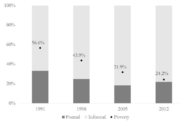

Share of formal sector workers out of all employed and self-employed (15 years or older).
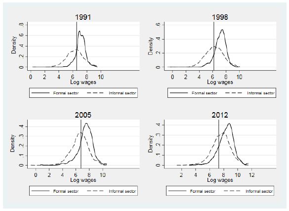

Wage distribution of formal and informal workers across time.
4. Modelling approach
For the purpose of this study we combine econometric estimation methods and microsimulation methods which are explained in more detail below. The results from both methods inform each other in the following manner: first, we estimate the elasticity of the formal sector with regard to the net pay difference between the formal and the informal sector based on four waves of the GLSS. Second, we use GHAMOD, the microsimulation model for Ghana, to simulate two different policy reforms: a stand-alone expansion of social protection and a revenue-neutral expansion of social protection financed through an increase in employee payroll tax. Next we combine the changes arising in the net pay differential between the formal and informal sector due to the policy changes with the formality elasticity estimated in the first step, to gauge the effect on the size of the formal sector. Finally, we recalibrate the weights taking into account the changes in the size of the formal sector, before calculating the overall effects of the policy and behavioural changes on poverty and distributional outcomes and the government budget.
4.1 Conceptual framework
We consider the following stylized framework to form the backdrop for the econometric work. The individual can either work in the formal sector, earning income yf, or in the informal sector (or in the shadow economy), earning income ys. If the individual works in the formal sector, he or she pays taxes (which can include employees’ social security contributions) T(yf) and obtains transfers equal to B(yf). Thus, net income in the state of formal work is given by xf = yf − T(yf) + B(yf), which must be sufficient to finance consumption cf (1 + τ), where τ is the consumption tax rate. Note that payroll taxes paid by employers affect the gross salary. The labour costs to the employer, denoted by Yf, are Yf = (1 + p)yf, which means that the gross income already encompasses the erfect of payroll taxes, as gross income can also be written as
If the individual works in the informal sector, no taxes are paid, but the individual might still be entitled to some benefits, B(ys), reflecting the fact that social protection programmes in developing countries, including in Ghana, often reach those working outside of the formal sector. The net income in the state of informal work is thus xs = ys + B(ys), which is used for consumption cs(1 + τ). Note that here we assume that both those in the formal sector and those in the informal sector indirectly pay value-added tax. Those who do not work at all can be treated as informal sector workers, but earning zero labour income.
The individual utility is linear (or log-linear) in consumption, and utility when working in the formal sector is thus xf/(1 + τ) − ψ, where ψ is the cost (which can be negative) of working in the formal sector. The costs are positive if working in the formal sector requires for instance a longer commute but the costs can also be negative, if formal sector work also brings about other benefits (such as retirement income). The utility when working in the informal sector is xs/(1 + τ). This means that the individual works in the formal sector if
which also means that the commodity tax does not affect the choice between formal and informal sector work.
Note that although this model is written as if working in the formal versus informal sector were solely based on individuals’ choice it can also be interpreted from the perspective of employers: the taxes on formal work create a wedge for formal sector employers, and any tax changes therefore reflect in the gross wage employers offer. According to conventional economic incidence analysis, a reduction in the income tax paid by workers can lead to a reduction in their asking wage, and therefore increase employment. Such a mechanism is, however, not possible, if the tax cut affects workers whose employment probability is distorted by the presence of a minimum wage. For such workers, even if a tax cut would lead them to be satisfied with a lower gross wage, this would only lead to an increase in the supply of labour and not to an increase in employment (which is restricted by the minimum wage).7 It is for this reason that in the estimations below we mostly focus on workers who are paid wages above the legally binding minimum wage. Another potential complication would arise from general equilibrium effects on wages—gross pay could be a function of the changes in the number of workers, but as in most micro-econometric tax studies such issues are assumed away in the basic set-up.
4.2 Estimation
In the empirical approach, explained in more detail in the Appendix, the idea is to estimate an empirical counterpart of Equation 1, that is the probability of working in the formal sector P(yf > 0)i,t for the individual i and at period t is
where P(yf > 0) is defined to take on the value of 1 if the individual supplies labour income in the formal sector exceeding zero. The estimation of equation (2) raises a number of challenges. One is that the key regressor on the right, (xf − xs), is endogenous: if a person moves from the informal to the formal sector, net income changes. Second, net income is only observed for one state (informal/formal) at a time. The solution is to utilize a group-based pseudo panel approach, where the data are aggregated to groups, defined based on exogenous characteristics (such as sex, age, education), and the equation is estimated at a group level. Then, group mean values are used to get an estimate for (xf − xs) for each individual. The approach can also be interpreted as an instrumental variables approach, where group-time interactions are used as excluded instruments for (xf − xs) in a model with group and time fixed effect added to an equation like (2).
The results can be converted into an elasticity format, where the elasticity of the share of formal work with respect to the change in the net pay (xf − xs), or formality elasticity for short, is defined as
4.3 Data and estimation results
We use waves 3 to 6 of GLSS for the estimation. The data are divided into groups based on sex, age (five ten-year age groups for persons between 15 and 60 years of age), and four education groups.9 The data are restricted to those who are workers; that is the self-employed are dropped from the estimation sample.
Elasticity of the share of formal work with respect to the change in the net pay between formal and informal work.
| No controls | All controls | All controls, above minimum wage | |
|---|---|---|---|
| Elasticity | 0.265** | 0.081 | 0.106 |
| Std error | 0.106 | 0.052 | 0.064 |
| Number of cells | 101 | 101 | 94 |
-
Source: Authors’ calculations based on GLSS data.
-
Notes: Linear probability regression results with the share of formal work as the dependent variable. The key regressor is the difference between the log of net pay in the state of formal work versus the log of net pay in the state of informal work. The model in Column 1 with no controls, the model in Column 2 with a full set of group and time dummies (groups formed based on age, sex, and education), and the model in Column 3 with the wage restricted to lie above the legal minimum wage. Instead of the regression coefficient, an elasticity estimate is shown. Standard errors calculated with the delta method.
-
*
indicates significance at the 10% level and *** at the 1 per cent level.
The result for models where log of net income is used are reported in Table 2. The first column shows only the strong correlation between the share of formal work and the difference in the take-home pay between formal and informal work, the second model includes a full set of group and time dummies, and the final column is the preferred specification, where the formal sector wage is restricted to be above the minimum wage. The results from the final two models can be given a causal interpretation. The result in Column (3) is statistically significant (at the 10 per cent level) and the estimated elasticity is not too far away from the ballpark of extensive margin elasticities estimated using high-income country data. The results reported here differ somewhat from those in McKay et al. (2018), due to a small difference in the way formality is defined. If the self-employed were included, the elasticity would increase (from 0.10 to 0.15 in Column 3 of Table 2), but the statistical significance would drop.10
4.4 Simulation of tax-benefit reforms in Ghana
4.4.1 GHAMOD, a microsimulation model for Ghana
Our starting point is the static tax-benefit microsimulation model, GHAMOD Adu-Ababio et al. (2017). The model is built on the EUROMOD platform. The underpinning data set is the latest wave of the GLSS, wave 6 from 2012/13. The policy rules are modelled for every year from 2013 to 2016; from 2014 on, all incomes are uprated taking into account inflation, though exclusively using the Consumer Price Index due to lack of other indices. For the purpose of this study all simulations are performed for the base year, 2013, and no uprating is necessary. GHAMOD is freely available for non-commercial research purposes.11
The model simulates the following taxes, levies, and benefits:
Personal income tax, which is a progressive tax on income from formal work with a top marginal tax rate of 25 per cent.
Social security contributions are a combination of two schemes. The SSNIT (Social Security and National Insurance Trust) rate is a flat-rate tax levied on employers and employees in the formal sector and restricted to those aged 15 to 45 years. The SSNIT rate is 5.5 per cent for employees and 13 per cent for employers. There is no minimum or maximum payable amount.
The LEAP transfer programme, which is geared towards extremely poor households (consumption per adult equivalent of GHS446) that also serve as caregivers to orphans or vulnerable children or have a pregnant, disabled, and/or old (65 or older) member. The total benefit paid to the household increases with the number of qualified individuals in the household from GHS8 for one qualified individual, GHS10 for two, GHS12 for three, and GHS15 for four or more qualified individuals.
A school feeding programme (or its monetary equivalent, as it is an in-kind transfer).
The value-added tax.
All excises.
Simulations of indirect taxes are based on the reported expenditures in the household data set.
4.4.2 Policy reform scenarios
We model two different policy scenarios: (1) a stand-alone extension of social protection (Reform A) and (2) a revenue-neutral scenario where the more generous social safety net introduced is fully financed through an increase in employee payroll tax (Reform B). Both scenarios extend existing policies, namely the LEAP benefit and the SSNIT rate for employees.
In policy scenario (1) eligibility conditions for the LEAP transfer are relaxed and the benefits made more generous:
The benefit amounts are raised to the level that came into effect only in 2014, more than tripling benefit amounts with the minimum benefit increasing from GHS8 to 32 and the maximum benefit from GHS15 to 53 a month per household.
The household eligibility condition is made more generous. Households with consumption between the initial threshold (that is the GHS446 line) and twice that amount (GHS 892) are now also eligible if fulfill-ing the individual conditions. For those below the initial threshold the amounts of the reform scenario are further doubled. Thus, a household below the GHS446 line and with one qualifying individual would receive GHS64 in the reform scenario compared to the GHS8 under the rules actually in force in 2013.
Introduction of a universal old-age pension: households with individuals aged 65 and over who do not receive any other pension become eligible to the benefit amounts spelt out under the first bullet point.
All households with under-age children (under 18 years of age) which fall below the GHS892 threshold are eligible, not only those households caring for orphans or vulnerable children.
The different elements of reform A are simulated together in the same reform scenario. The order of the simulation is such that the pension reform takes place first, as it can have an impact on eligibility for some LEAP transfer recipients. Reform scenario A disregards entirely how such rather massive extension could be financed.
Reform scenario B in turn is designed to fully finance the costs accruing to the government when extending social protection: on the benefit side the same rules as under scenario (1) apply. Additionally, the SSNIT rate for employees is raised to the point that it can recoup the costs of the LEAP expansion assuming no behavioural change. The increase in the SSNIT rate necessary to offset the additional expenditure on the reformed LEAP transfer programme assuming no behavioural adjustments is eight percentage points. The exact change in the tax rate depends, of course, on how well the baseline simulation matches the actual tax receipts reported by the government. The background study by Adu-Ababio et al. (2017) reports results from a macro validation, where the total tax revenue as predicted by GHAMOD is compared with information on actual revenues from the Ministry of Finance. The simulation of labour income tax (totalling GHS2.1 billion), for which external information exists and whose base is close to the social security contributions base, is reasonably close to the officially stated receipts (GHS2.4 billion).
We chose to finance the additional social protection through increasing the payroll tax as changes are easy to implement and straightforward to understand. By contrast, changes to progressive income tax rate schedules are more intricate. Clearly, financing the reform with increases in indirect taxes would also be an option. Yet in the absence of consumption data revealing whether the households use informal versus formal retailers to purchase goods, changes in indirect taxation would not have any impacts on the formality margin.
5. Results
The results are reported in Tables 3 and 4. In the first column, we report the baseline/status quo results for the year 2013. Poverty and inequality are measured using consumption. As the changes in the policy experiment refer to income changes, we turn these into changes in consumption possibilities. In other words, we examine how much consumption would change if all the additional income were spent. The next two columns are based on static microsimulation with no behavioural impacts. The first of these shows the impacts of expanding the social protection alone (Reform A: non-revenue-neutral scenario) and the second the impacts of a reform where the SSC paid by the employees is raised to recoup the revenue (Reform B: revenue-neutral scenario). The last column includes the results with the behavioural impacts, thus where the tax increase leads to a reduction in the share of formal work (Revenue-neutral reform with behavioural impacts).
Simulation results of expanding social protection on poverty and inequality.
| Status quo | Reform A: Stand-alone extension of social protection | Reform B: Revenue-neutral reform | Revenue-neutral reform with behavioural impacts | |
|---|---|---|---|---|
| (I) | (II) | (III) | (IV) | |
| FGT(0) | ||||
| All | 24.9 | 24.1 | 24.3 | 24.4 |
| Male-headed households | 26.6 | 26.0 | 26.2 | 26.3 |
| Female-headed households | 19.7 | 18.4 | 18.5 | 18.6 |
| Households with children | 27.4 | 26.7 | 26.9 | 27.0 |
| Households with older persons | 33.7 | 29.3 | 29.3 | 29.4 |
| FGT(1) | ||||
| All | 8.1 | 6.7 | 6.8 | 6.8 |
| Male-headed households | 8.8 | 7.3 | 7.5 | 7.5 |
| Female-headed households | 6.0 | 4.6 | 4.7 | 4.7 |
| Households with children | 8.9 | 7.4 | 7.5 | 7.5 |
| Households with older persons | 11.0 | 7.8 | 7.9 | 7.9 |
| Gini | 41.7 | 40.8 | 40.8 | 40.8 |
| P80/P20 | 3.53 | 3.46 | 3.46 | 3.46 |
-
Source: Authors’ calculations based on GHAMOD v1.0.
-
Notes: Poverty rates measured using the consumption-based absolute poverty line of GHS 1,314 per adult equivalent per year. The Gini index is also calculated on the basis of consumption.
The labour supply estimates reported in Table 2 suggest an elasticity of 0.10 (Column 3). When calculating the impacts of the reduction in the share of formal workers we assume that the larger number of workers in the informal sector does not change informal sector wages. While there is of course concern for more general equilibrium effects, we consider the effects of the proposed interventions on labour supply in the informal sector to be not important enough to exert downward pressure on wages in the informal sector.
In a revenue-neutral reform scenario government needs to increase the general component of the SSNIT contribution by eight percentage points (from 3 per cent to 11 per cent).12 The decrease in the difference in net wages between the formal and informal sector wage together with the elasticity estimated in Table 2 then implies that formal sector work is decreased by approximately 1 per cent.
Reforming LEAP and the pension system reduces poverty overall (Column 2), and in particular among households with older persons (defined as households with at least one member above 65). While the headcount rate (FGT(0)) overall would decrease by less than one percentage point in the reform scenario, it would decrease by more than four percentage points among households with older persons. Female-headed households also benefit slightly more than male-headed households. The wide coverage of the simulated pension benefit explains why households with older persons benefit particularly. The poverty gap index (FGT(1)) is reduced relatively more, especially among households with older persons. The decrease in poverty is accompanied by a decrease in inequality as the proposed reform of the benefit system mainly benefits those at the bottom of the income distribution.
In a revenue-neutral reform scenario (Column 3 of Table 3) these effects remain largely the same: the decrease in poverty is smaller overall but still sizeable for households with older persons. Interestingly, the effects of the proposed reforms remain stable even when considering negative effects on the share of formal sector workers due to higher social security payments by employees in the formal sector (Column 4 of Table 2); the decrease in the formal labour share barely affects poverty rates as households benefiting from the increased social protection are mostly employed in the informal sector.13
Changes to the government budget based on the simulated social protection expansion.
| Status quo | Reform A: Stand-alone extension of social protection | Reform B: Revenue-neutral reform | Revenue-neutral reform with behavioural impacts | Difference between (III) and and (IV), in % | |
|---|---|---|---|---|---|
| (I) | (II) | (III) | (IV) | ||
| LEAP benefit | 3.3 | 273.5 | 273.5 | 273.8 | 0.09 |
| Old-age LEAP | 0.0 | 436.6 | 436.6 | 436.7 | 0.02 |
| Employee SSC | 485.6 | 485.6 | 1191.9 | 1179.7 | −1.02 |
| Employer SSC | 1066.5 | 1066.5 | 1066.5 | 1055.7 | −1.02 |
| Income tax | 2059.8 | 2059.8 | 2059.8 | 2038.8 | −1.02 |
| Budget effects | - | 706.7 | 3.8 | 44.8 | - |
| Formal sector (%) | 13.6 | 13.6 | 13.6 | 13.5 | −0.88 |
-
Source: Authors’ calculations based on GHAMOD v1.0.
-
Notes: The budgetary implications are expressed in millions of GHS.
The proposed reforms entail significant costs to the government’s budget (see Table 4). Extending coverage of LEAP increases expenditure on the LEAP programme by more than 120 times (Column 2 in Table 4). Extending coverage of the pension system to those aged 65 years and above with no pension entitlement so far implies additional expenditures of GHS 437 million. Both reforms together thus amount to a total of GHS 710 million of additional expenditure for the state budget. In a revenue-neutral setting, on the other hand, government more than doubles its income from employee SSC (from 486 to 1192 GHS million, Column 3 in Table 3) to offset the additional expenditure due to the extension of social protection.14
Factoring in behavioural responses of labour supply (Column 4 in Table 3) shows that the consequences of a lower share of formal sector employees for the state budget are negative but not drastically so. The government now has lower receipts of employee SSC, due to the smaller formal sector, but the decrease is overall around 1 per cent. The receipt of employer SSC and income tax is reduced by a similar amount in the scenario with behavioural responses.
5.1 Sensitivity analysis
The purpose of this section is to examine how sensitive the results in the analysis with behavioural impacts are with respect to some key parameter values. Equation 3 implies that the change in the share of the formal sector, dP(yf > 0), relates to three factors, namely the initial size of the formal sector, P(yf > 0), the relative change in net pay, d(xf − xs)/(xf − xs), and the elasticity of formality regarding the change in net pay, ε. Specifically, the share of the formal sector increases in (i) the initial size of the formal sector, (ii) the relative change in net pay, and (iii) the elasticity of formality. The difference in the poverty and government budget implications of the reform between the static and dynamic calculation is therefore directly related to the magnitude of these three terms. Out of these, we would argue that the first, the share of the formal sector, is fairly reliably measured in the data; our estimate of its size is also close to external information from Alagidede et al. (2013). We therefore conduct sensitivity analysis with respect to the latter two parameters, the elasticity of formality and the change in the net wage.
The formality elasticity (approximately 0.10) is modest, and therefore it is worth investigating how much the results would change if one were to use a higher elasticity estimate. We therefore repeat the calculations by assuming an elasticity equal to 0.75. We also experiment with changing the relative change in net pay (which is around −10 per cent in the base analysis). One could argue that using mean values of net incomes for all formal and informal sector workers could overestimate the wage difference between the two sectors, if for instance a high proportion of informal sector workers are relatively immobile rural agricultural workers with low pay. This would, in turn, underestimate the relative change in the net pay when taxes are increased. A more detailed analysis of the data reveals that the pay difference across sectors is indeed somewhat smaller in urban areas. However, the urban formal sector gross wage is also higher on average, implying that the relative change in net pay is approximately −13 per cent when calculated among the urban sector workers only. This reasoning led us to check the implications of using a −15 per cent change in the net pay in the dynamic analysis.
The results for government revenues and expenditures are reported in Table 5. The costs of the reform increase significantly, especially in the case where the elasticity is increased: the government budget has a shortfall of more than GHS 300 million instead of the GHS 45 million in the dynamic baseline calculation (Column 3 compared to Column 1). The increase in the size of the net pay change has a more muted impact on the costs, but of course, the magnitude of the changes made to parameter values were much more significant when changing the elasticity.
We have also calculated the impacts of these changes to the reform on poverty and inequality (not shown for brevity). The results remain almost the same, with the Gini dropping to 40.7 and the poverty impacts the same at the one-digit level. Of course, if one needed to further increase the tax rates to return to a revenue-neutral scenario, the poverty rates could also increase. Despite this caveat, the main pattern of the results seems to be fairly robust; even when taking (larger) behavioural changes into account, the reform appears to reduce poverty and inequality.
Ideally, one should also examine whether the results in various scenarios are different in a statistically significant manner, as proposed in the paper by Goedemé, Van den Bosch, Salanauskaite, and Verbist (2013). However, in our case examining this issue would not be straightforward, since the statistical inference analysis would also need to cover the estimation part. We therefore leave this for future analysis.
Sensitivity analysis of government revenues and expenditure.
| Revenue-neutral reform with behavioural behavioural impacts | As (I) with greater wage change (-0.15% instead of −0.10%) | As (I) with higher elasticity (0.75 instead of 0.1) | |
|---|---|---|---|
| LEAP benefit | 273.8 | 273.9 | 275.4 |
| Old-age part of | 436.7 | 436.7 | 437.3 |
| LEAP benefit | |||
| Employee SSC | 1179.7 | 1174.0 | 1100.6 |
| Employer SSC | 1055.7 | 1050.5 | 985.9 |
| Income tax revenue | 2038.8 | 2028.9 | 1902.1 |
| Change in costs vs. | 44.8 | 65.7 | 333.6 |
| status quo | |||
| Share of formal workers (%) | 13.5 | 13.4 | 12.7 |
-
Source: Authors’ calculations based on GHAMOD v1.0.
-
Notes: The first column reproduces the numbers of Column (4) in Table 4.
6. Conclusion
This paper has studied, for the first time to our knowledge in a developing-country case, the impacts of expanding social protection and financing it using a tax-benefit model with behavioural elements. For the latter part, we presented estimates that identify the causal impact of tax changes on the share of formal work in Ghana. These estimates were then taken into account in the simulation and the overall impacts were calculated for the case both with and without behavioural changes.
The simulated policy included expanding the amounts and the eligibility threshold of the existing LEAP cash transfer programme and introducing a new universal old-age pension. The amounts offered in these reforms are still very modest and they alone would not raise the households above the poverty line. This is why their estimated impact on the poverty headcount rate was also fairly small: less than a one percentage point reduction for households with children and a four percentage point reduction for households with older people. The cost of the programme would be approximately GHS 700 million and financing it with an increase in the social security contribution of formal sector employees would imply raising the rate by approximately eight percentage points. The increase is sizeable, given the narrow base of the tax.
Our preferred estimate for the elasticity of the share of formal work with respect to the difference in the net pay when in formal versus when in informal work is approximately 0.10. It is statistically significant, albeit at the 10 per cent level, but also very small. This also means that the difference in the poverty-reducing impact of social protection when estimated with or without behavioural linkages is small. This finding is reinforced by the fact that poor households do not typically work in the formal sector and that is why they are not affected by the tax increase. The costs of financing the programme increase by approximately 6 per cent due to the reduction in the share of formal work.
A number of caveats need to be kept in mind when interpreting the results. First, the estimated elasticity could be larger, and we have carried out some sensitivity analysis with respect to the size of the elasticity. Second, since the data set was originally prepared to study consumption, the income data are not necessarily as reliable. Third, the poverty eradication effects would be greater if, instead of modelling the tax increase via the flat social security contributions, progressive income tax were used. One further issue is that all those working in the formal sector are modelled to pay taxes. However, while their income from their main job is subject to third-party withholding by employers, they can still evade taxes from other income they earn and, arguably, the extent of evasion may also depend on the tax rate. This means that the exact size of the tax rate increase is only estimated with some margin of error. As always in microsimulation models, we have not allowed for any “leakage” due to administrative costs or misspent revenues by the social protection administration: a point with perhaps more relevance in a poor-country context with more limited government capacity. Tackling many of these issues is on our future research agenda.
Footnotes
1.
More information about the project is available at https://www.wider.unu.edu/project/southmod-simulating-tax-and-benefit-policies-development.
2.
For information about EUROMOD, which is both a tax-benefit model for European countries and software for building microsimulation models, see Sutherland and Figari (2013).
3.
The estimator was used by Blundell, Duncan, and Meghir (1998) for the case of labour supply in the UK and applied to a cross-country case by Jäntti, Pirttilä, and Selin (2015).
4.
Comparability between the first two waves and GLSS 3 and later rounds is undermined by the differences in the survey method.
5.
Different characteristics between formal and informal workers may mean that finding a job in the formal sector is not easy for many informal sector workers, such as agricultural workers in rural areas. We will consider the consequences of this for the microsimulation results with dynamic effects towards the end of Section 5.
6.
Note also that any changes in the payroll tax that the employer needs to pay for the formal sector wage, (1 + s) y f, are already reflected in the gross pay, y f, depending on the incidence of payroll taxes.
7.
The minimum wage was 1452 per year in 2012.
8.
We acknowledge that this issue is more complicated in practice, as minimum wages are not necessarily effectively enforced: see Bhorat, Kanbur, and Stanwix (2015).
9.
The groups are: Not completed primary education, completed Primary, Lower secondary, and Upper secondary or higher.
10.
Our estimated elasticity appears to be somewhat smaller than the results in some studies using data from Latin America. For example, Kugler and Kugler (2009) using plant level data for Colombia find that a 10% increase in payroll taxes leads to reduction in formal employment of between 4 and 5%. The results in Bergolo and Cruces (2014) indicate that a one percentage point increase in net income implies an about 1.7% increase in registered employment.
11.
For more information, see https://www.wider.unu.edu/about/accessing-southmod-models.
12.
Due to a rounding error, the proposed reform is not exactly revenue neutral.
13.
The reason for the small difference between Columns 3 and 4 is that the change in the formal sector share is modest and those who lose a formal sector job are still employed (albeit with a somewhat lower wage).
14.
The reason that such a relatively costly reform leads to fairly small changes in poverty on average is explained by the fact that the total poverty gap (the number of poor persons times the mean poverty gap per person) was approximately GHS 8.7 billion, implying that complete poverty eradication would require reform of a greater order of magnitude.
15.
This section draws heavily on the material in Jäntti et al. (2015) and McKay et al. (2018).
16.
Appendix
As already mentioned in the main text, estimating Equation (2) poses a number of challenges.15 First, the right-hand side regressor is correlated with e and so endogenous. The most obvious reason is that both taxes and benefits are direct functions of income. An additional reason is that unobserved variables (for instance, tastes for work and savings) might affect the choice of working in the formal sector. Since the individual is only observed in at most one state at a given time, income in the other state needs to be imputed.
Our approach to tackling these issues is to utilize the repeated cross-section element of the data. This allows us to compare groups of individuals over time and, thereby, address these endogeneity issues by constructing instruments. Following Blundell et al. (1998), we partition the sample into group cells based on country, sex, age, and education level. The key idea behind the grouping procedure is to compare otherwise similar groups of individuals who have been affected differently by tax reforms (the difference-in-difference setting), while retaining the ambition of estimating structurally meaningful parameters, in this case the formality elasticity.
Let g denote group cell. Suppose that εit = αg + μt + ηit, where E[ηit\hit > 0,g,t] = 0. According to this assumption unobserved heterogeneity, conditional on g and t, can be captured by a permanent group effect αg and a time fixed effect µt. This assumption can also be modified in such a way that it allows for instance for education-group-specific linear time trends. Let ωgt be a vector that contains the full set of interactions between group and time. By assumption, these are uncorrelated with ηit. This is the central exclusion restriction for identification. We can then estimate
by two-stage least squares (2SLS) while using ωgt as excluded instruments for (xf − xs). The instrument needs to have sufficient predictive power and it must affect the outcome variable only via changing the net pay variable. As the variation in the second-stage equation is entirely at the group level, Equation A1 can also be estimated by collapsing the data into time-specific group averages of the relevant variables. We then estimate the parameters from
by GLS, using group size as weights. Using either Equation A1 or A2 yields identical results. Note that the estimation of the probability of working in the formal sector not only hinges on tax and benefit reforms, but is also identified from shocks affecting the gross pay in the two different states.
To deal with missing income in either of the states, we proceed using a simple and transparent approach utilizing cell means. We use the cell means
References
-
1
A tax micro-simulator for Mexico (MEXTAX) and its application to the 2010 tax reforms (IFS Working Paper (W15/23))London: Institute for Fiscal Studies.
- 2
- 3
-
4
Welfare programs and labor supply in developing countries: experimental evidence from Latin AmericaJournal of Population Economics 26:1255–1284.
- 5
-
6
Issues on wages and labour market competitiveness in GhanaIssues on wages and labour market competitiveness in Ghana, Accra.
-
7
Work and tax evasion incentive effects of social insurance programs: Evidence from an employment-based benefit extensionJournal of Public Economics 117:211–228.
-
8
Minimum wages in Sub-Saharan Africa: A primer (IZA Discussion Paper No. 9204)Bonn: Institute of Labor Economics (IZA).
- 9
-
10
The impact of a social program on labor informality: The case of AUH in ArgentinaJournal of Development Economics 115:99–110.
-
11
Ghana Living Standards Survey Round 6 (GLSS6): Labour Force ReportAccra: Ghana Statistical Service.
-
12
Ghana Living Standards Survey Round 6 (GLSS 6): Main ReportAccra: Ghana Statistical Service.
-
13
Testing the statistical significance of microsimulation results: A pleaInternational Journal of Microsimulation 6:50–77.
-
14
Estimating labour supply elasticities based on cross-country micro data: A bridge between micro and macro elasticities?Journal of Public Economics 127:87–99.
-
15
Labor market effects of payroll taxes in developing countries: Evidence from ColombiaEconomic Development and Cultural Change 57:335–358.
-
16
Estimating the elasticity of formal work: Evidence from African countries (Tampere Economic Working Papers No. 120)Tampere: University of Tampere.
-
17
Ghana: Poverty reduction over thirty yearsIn: C Arndt, A McKay, F Tarp, editors. Growth and Poverty in Sub-Saharan Africa. Oxford University Press. pp. 68–88.
- 18
- 19
-
20
EUROMOD: The European Union tax-benefit microsimulation modelInternational Journal of Microsimulation 6:4–26.
Article and author information
Author details
Acknowledgements
This paper is part of UNU-WIDER research programme on “Economics and Politics of Taxation and Social Protection”. Funding from the Academy of Finland (Grant No. 268082) is also gratefully acknowledged. We thank two anonymous referees and participants of the ZEW Public Finance Conference, UNU-WIDER seminar, 2017 PEGnet conference, the 2017 International Institute for Public Finance Conference, and the 2018 Conference of the Centre for the Study of African Economies in Oxford, for helpful comments. The results presented here are based on GHAMOD v1.0. GHAMOD was developed, maintained and managed by UNU-WIDER in collaboration with the EUROMOD team at ISER (University of Essex), SASPRI (Southern African Social Policy Research Insights) and local partners in selected developing countries (Ethiopia, Ghana, Mozambique, Tanzania, Uganda, Zambia, Ecuador, and Viet Nam) in the scope of the SOUTHMOD project. The local partner for GHAMOD is University of Ghana. We are indebted to the many people who have contributed to the development of SOUTHMOD and GHAMOD. The results and their interpretation presented in this publication are solely the authors’ responsibility.
Publication history
- Version of Record published: April 30, 2019 (version 1)
Copyright
© 2019, Osei et al.
This article is distributed under the terms of the Creative Commons Attribution License, which permits unrestricted use and redistribution provided that the original author and source are credited.