A care time benefit as a timely alternative for the non-working spouse compensation in the Belgian tax system
- University of Antwerp, Belgium
Abstract
Over the past decades, the growing labour force participation of mothers has rendered the Belgian personal income tax system increasingly outdated. Especially the ‘marital quotient’ system – that allows spouses with monetary income to transfer part of their tax base to a spouse without monetary income – is no longer a tax allowance that compensates childcare efforts. It rather has become a subsidy to older cohorts for their past childcare efforts. As an alternative, we model in this article a system that is geared towards the effective care trajectories of nowadays parents. We thereby follow earlier ideas of Hilde Bojer, Patricia Apps and Ray Rees to reflect care efforts in the tax base of individuals. Following Bojer, we propose a system that incorporates a socially grounded amount of childcare time in household income, and simulate this with the Belgian microsimulation model MISIM. The amount relates to the number and age of children and can either be procured through childcare services or self-provision. In the proposed system both market- and self-provided care result in a similar subsidy. We elaborate a monetary estimate of self-provided childcare on the basis of the detailed information of time use in the Flemish Family and Care Survey (2004-2005). For discussion we provide an overview of potential drawbacks and advantages and evaluate the redistributive impact of the simulated alternative.
1. Introduction
Over the past decades, the growing labour force participation of mothers has rendered the Belgian personal income tax system increasingly outdated. Especially the ‘marital quotient’ system – that allows spouses with monetary income to transfer part of their tax base to a spouse without monetary income – is no longer a tax allowance that compensates childcare efforts. It rather has become a subsidy to single income couples, often belonging to older cohorts. In the framework of increased policy attention for reconciliation of family and work, one can ask whether the considerable budget used for the marital quotient cannot be used in a more ‘childcare-friendly’ way.
In this article we investigate the possibilities of reforming the personal income tax system in such a way that it is geared towards the effective care trajectories of nowadays parents. We thereby follow earlier ideas of Hilde Bojer (2006), Patricia Apps and Ray Rees (2001) to reflect care efforts in the tax base of individuals. Following Bojer, we propose a system that incorporates a socially grounded amount of childcare time in household income. The amount relates to the number and age of children and can either be procured through childcare services or self-provision. In the proposed system both market- and self-provided care result in a similar subsidy, and is therefore neutral with respect to this choice.
This article is organised as follows. First, we picture the current policy context with regards to the reconciliation of work and family and the income tax system and argue why the current ‘marital quotient’ system should be abolished. Next, we elaborate the concept of ‘socially grounded childcare time’ as a way to allocate a care allowance in a socially justified manner. Subsequently, we discuss our data, the tax- benefit model MISIM and the methodological issues of our policy simulation. The next section presents the results of the simulation exercise regarding household income, income distribution and poverty. We thereby pay specific attention to winners and losers with respect to the current situation and estimate the size of the impact. Finally, we round up with a summary and conclusion.
2. Socially grounded child-care time as an element of belgian income tax
The growing lack of congruency between the Belgian personal tax system and the degree of labour force participation of mothers, is most clearly exemplified in the ‘marital quotient’ system1 This system was introduced in the 1988 tax reform with the stated aim to restore the neutrality of the choice between professional and domestic work. The ‘marital quotient’ means that for single-income couples a proportion of the professional income of the earning spouse can be transferred to the non-earning spouse (for more details see Section 3.4). The part transferred to the other spouse is then taxed separately, in general at a lower rate. Thus, to foster neutrality of choice, the system allows a tax advantage to couples with one spouse without (or with a low amount of) professional earnings. It thereby supposes that these spouses are engaged in care work. Yet, with the growing employment rate of Belgian mothers, the system has to a large extent transformed into a subsidy to older cohorts for their past childcare efforts rather than a compensation for childcare efforts of the current generation of parents (Verbist, 2002).
Therefore, we propose, as an alternative, a system that is exclusively geared towards the effective care efforts of nowadays parents. We thereby draw on earlier ideas of Hilde Bojer (2006) and Patricia Apps and Ray Rees (2001) about the incorporation of care efforts in the tax base of individuals. Apps and Rees (2001) argue that thinking about the ‘cost of children’ and especially about its compensation in tax or social security systems has been largely geared towards the market consumption costs, while the value of time represents a more important parental effort2. They therefore propose to incorporate the value of household production, as a result of market inputs and parental time, in household wealth.
Bojer (2006), on the other hand, applies Amartya Sen’s capability approach to argue that to achieve social inclusion parents are to make specific efforts to care for their children. Society depends on parents for the raising of the future citizens and develops a set of socially sanctioned expectations (‘norms and values’) to guarantee the proper upbringing of its members. Therefore, by having children, parents are socially constrained in their time allocation and can no longer realize their full income in the sense of Becker (1991). In other words, while the budget constraint of non-parents is constrained only by physiological limits to human effort, parents face an additional constraint imposed by social expectations regarding the upbringing of children. Parents are free to choose the exact mix of own childcare time and childcare services, but both options curtail the potential private income, either by a time constraint or by expenses on these services. Note, however, that Bojer (2006) does not suggest to value the loss in potential private income through the effective care efforts of parents, but following Sen, proposes to determine a socially grounded amount of childcare effort through a democratic procedure. This means that parents receive a kind of childcare time entitlements according to the ruling social norms. In practice, most parents will spend either more or less time on their children than this norm, but this is their personal decision and they will not be compensated for a possibly larger effort3.
Following Bojer, we propose a system that incorporates a socially grounded amount of childcare time in household income.4 The amount relates to the number and age of children and can either be procured through childcare services or self-provision. In our proposed system the parental subsidy is independent from whether the childcare is market- or self-provided, because it is the total time effort that counts. The optimal mix of both is left to the parent(s), who are likely to decide on the basis of their preferences and the opportunity costs of the alternatives.
Note, finally, that our proposal leaves several parts of the Belgian tax system untouched, even though they are child related. Most importantly, in our simulation of alternatives we do not alter the current rules that raise the non-taxed part of the household income in function of the number of children. Neither do we modify the system of child benefits. We leave both in place because they account for the market consumption costs of child raising, which goes beyond the scope of the present analysis.
3. Methodology
3.1 Data
The European Union Survey on Income and Living Conditions (SILC) of the survey year 2004 (with income data referring to 2003) provides the micro data (Federale Overheidsdienst Economie, 2006). The Belgian SILC-2004 has 5,275 households and 12,971 individuals. Apart from the standard socioeconomic data (income, household composition, etc), this dataset contains specific data on childcare which are particularly relevant for our analysis. In 2004 there was a detailed set of questions on type of childcare (both formal and informal), as well as on the time spent by each child in these types. Unfortunately, the SILC data do not provide information on parental out-ofpocket payments for childcare. These are derived from the Flemish Family and Care Survey (FFCS), which was conducted in 2004/2005. The FFCS was elaborated to provide data for micro-distribution analysis of families with children in Flanders and provides data on income sources, expenses, care needs and the use of care services of families with children. We base our analyses on a representative sample drawn from the population register. Within this sample 474 families are effective users of child care services and have provided full information on child care costs and the time use of their children. The information in FFCS applies only to Flanders. As there is no similar data available for the other parts of the country, we assume that the information for Flanders is representative for Belgium as a whole. Below, we will discuss the degree of realism of this data driven assumption for every element of information we use from the FFCS.
3.2 Microsimulation model MISIM
For our simulation purpose, we use the microsimulation model MISIM (see Verbist, 2003). MISIM (MicroSImulationModel) is a static tax- benefit model, which enables to evaluate policy alternatives in the field of social security and personal income taxation. The model covers personal income taxes, social security contributions and part of social benefits. For this simulation, we need the personal income tax modules. In a first step taxable income is calculated, which includes professional income (both from self-employment and for employees) and social benefits, and interfamily transfers like alimony payments. As the cadastral income is not included in the first years of EU-SILC, real estate can unfortunately not be included; for more recent years cadastral income will be part of the Belgian version of SILC, thus enlarging the scope for potential simulations. The following tax deductions are applied on taxable income: professional expenses (at the rates provided in the tax law) and childcare fees. Next, the tariff structure is applied, as well as the tax credits for family composition, for replacement incomes and for long-term savings (to the extent that EU-SILC provides information on this last topic). As documented in Verbist (2002 & 2003), the Belgian personal tax system is well covered by MISIM, and outcomes are in line with administrative tax information.
As the personal income tax system is modelled with enough detail, we are able to simulate the effect of abolishing the marital quotient and the tax deduction for childcare expenditures. MISIM can provide as output both budgetary consequences of policy measures as well as the current distributive and poverty indicators. In this article, only first-order effects are considered, so no account is taken of possible labour supply effects.
3.3 Estimation of socially grounded amounts of child care
We argued in Section 2 that a compensation for the loss of personal income stemming from childcare which is both democratically legitimate and choice-neutral, should rely on a measure of socially required childcare time. Consequently, our measure requires the observation of two elements: the potential working time that parents have at their disposal and the part of this time that they are expected to provide childcare, either by themselves or through childcare services.
To fix the amount of hours that reflects the potential working time of parents, various assumptions are possible. Following the full income idea of Gary Becker (1991), one might choose all non-sleeping time in a week as reference and use, for example, 112 hours as the reference time, assuming 8 hours of sleep per day and 7 days a week as potential working days.
However, 112 hours a week is an amount that diverges strongly from the generally accepted working times in the society at hand and, hence, would set a reference that is not democratically legitimate. In fact we are looking for an amount of time that an individual could be working for pay while still being considered a responsible citizen. obviously, societies expect citizens to engage in more activities than paid work and sleep alone and, consequently, a socially accepted amount of potential working time cannot be as high as 112 hours a week. Therefore, we will rather use the distribution of actual working times as a reference for our estimate.
Moreover, we limit our attention to the time spent on paid employment by fathers in dual-earner households, the modal household type among parents in Belgium which we consider to function as the social reference. We exclude women and adults in single-earner families, because the majority of them are likely to exhibit constrained labour market behaviour. It is well known that a large part of mothers restricts paid employment because of care responsibilities, which makes the distribution of their actual working times an unsuitable basis for the estimate of what society considers to be acceptable yet maximised labour market attachment of parents. Likewise, men in single breadwinner families are likely to reflect in their choices the particular situation of their household (a non-working spouse or single parenthood), which may again render the distribution of their working times less suitable as an estimate of potential working time.5
Theoretically, one might also argue that single men and women without children might provide the most clear-cut references for unconstrained labour market behaviour. Here, we obtain the observed working times from the FFCS-database, which contains a weekly work schedule for a representative set of parents only.6
The following table describes the distribution of the time fathers declared to have spent on paid employment during a randomly chosen observation week, outside of traditional holiday periods.
The distribution of paid employment among fathers in dual-earner families, hours per week.
| N(observations) | 574 |
|---|---|
| Mean | 43h11’ |
| Percentiles | |
| 10 | 25.0 hours |
| 25 | 38.0 hours |
| 50 | 42.5 hours |
| 75 | 51.0 hours |
| 90 | 60.0 hours |
| 95 | 68.0 hours |
-
Source: FFCS (2004–2005).
-
Note: the original measurement is in half hour units.
We propose as a the social reference value the median 7 of the actual distribution, namely 42.5 hours per week, which is slightly higher than full time paid work as agreed by collective agreements for blue collar workers8. In other words, we set a weekly amount of 42.5 hours as social reference for potential working time for any parent in Belgium. For sensitivity testing we have also elaborated micro-simulations with a reference of 60 hours per week, which corresponds to the 90% value of the distribution and may come closer to the idea of full income (socially acceptable, yet maximised working time). As the results were hardly different from the 42.5 hours scenario, these are not presented in the article.
In practice, parents will determine how much of their potential working time they can actually spend on it, taking into account their preferences and the material and immaterial constraints they find themselves confronted with. The care requirements of their children play undoubtedly an important part in the latter. However, society assumes part of these care requirements in a universal way through the schooling system. Therefore, parents do not need to organise care for their children for the full period of their potential working time, but only for the part of the latter that is not covered by the schooling system.
In Table 2 we show some descriptive information about the time parents declared their children to be at school during a randomly assigned week during the school year 2004–2005. The table clearly reflects the high enrolment rates of toddlers in the Belgian preschool system. 9 As of the age of two and a half Belgian toddlers can attend preschool classes that form part of the schooling system and are fully subsidized by the state. By the age of three, enrolment is almost 100%, but full time attendance follows only later. The latter becomes nearly universal around the age of 5, i.e. one year before the start of primary school (the start of compulsory education).
Obviously, the survey results in the table reflect all types of school attendance in the observation week, including the lack of attendance due to illness. Consequently, it may not be a surprise that zero values occur at all ages, which explains why the mean values lie systematically below the median values. Moreover, the time registration did not distinguish between schooling time related to class attendance and care provided by schools before and after class times. While the first is universal and free of charge for parents, the second is only used by a fraction of parents (and children) and is charged to parents as any type of formal childcare service.
To avoid measurement errors, we therefore propose to use as estimate of the universal care offered by the Belgian schooling system the smoothed figure shown in the last column of Table 2. This figure reconciles the characteristics of the Belgian schooling system presented above with the observational results of the survey.10
Time spent at schoo1 according to the age of the child, hours per week.
| Age | Median | Mean | S.E. | Minimum | Maximum | N | Proposal |
|---|---|---|---|---|---|---|---|
| 0 | 0.00 | 0.00 | 0.00 | 0.00 | 0.00 | 45 | 0 |
| 1 | 0.00 | 0.23 | 0.17 | 0.00 | 9.75 | 69 | 0 |
| 2 | 0.00 | 6.52 | 1.48 | 0.00 | 43.42 | 60 | 0 |
| 3 | 24.96 | 22.49 | 1.63 | 0.00 | 40.00 | 46 | 25 |
| 4 | 28.43 | 27.25 | 1.30 | 0.00 | 49.75 | 46 | 28 |
| 5 | 31.50 | 29.66 | 1.05 | 0.00 | 46.50 | 61 | 30 |
| 6 | 30.42 | 28.57 | 1.23 | 0.00 | 43.00 | 40 | 30 |
| 7 | 29.49 | 27.06 | 1.16 | 0.00 | 43.17 | 62 | 30 |
| 8 | 33.36 | 34.99 | 1.92 | 13.50 | 103.50 | 58 | 30 |
| 9 | 29.00 | 25.92 | 1.03 | 0.00 | 39.75 | 73 | 30 |
| 10 | 26.75 | 22.60 | 1.66 | 0.00 | 40.50 | 49 | 30 |
| 11 | 30.55 | 27.68 | 1.21 | 0.00 | 41.67 | 66 | 31 |
| 12 | 30.75 | 27.01 | 1.62 | 0.00 | 43.17 | 55 | 31 |
| 13 | 35.50 | 32.12 | 1.46 | 0.00 | 52.75 | 69 | 32 |
| 14 | 26.00 | 25.02 | 1.83 | 0.00 | 45.75 | 51 | 32 |
| 15 | 33.50 | 27.88 | 1.63 | 0.00 | 53.00 | 74 | 32 |
-
Source: FFCS (2004–2005).
-
Note: the original measurement is in half hour units.
We make the concept of a socially grounded amount of child care operational by subtracting the time children spend at school from the potential working time of a parent. 11 For families with more than one child, the resulting care hours for each child are added up, to reflect the additive nature of market childcare costs. This results in the following monthly amounts of socially grounded child care.
3.4 Allocation of parental childcare ‘subsidy’
Our reform consists of the introduction of a parental childcare subsidy. This subsidy is funded through the abolition of the marital quotient and the transfer of personal tax allowance between married partners in the personal income tax system on the one hand and of the tax deduction for childcare fees and children younger than 3 on the other. The amount of the childcare subsidy is determined in such a way that the entire operation is revenue neutral, leaving government funds unaffected.
Concerning the category of rules allowing transfers between the partners, we opted to discard both the marital quotient system as well as the transfer of personal tax allowance between partners. Both rules can be considered as traces from the former joint taxation system, and were installed with the 1988 tax reform as a compromise regarding the single earner households. The marital quotient allows treating 30% (with a maximum amount of €8,030, tax year 2004 12) of total professional income of both spouses as the personal income of the nonworking spouse. As a consequence of the progressivity of the Belgian tax rates, this amount is taxed against the lowest marginal tax rate instead of against the higher rate of the bracket in which the single earner’s income would end up when treated as one entity. Abolition of the marital quotient can be considered as a further step in the individualisation of the personal income tax system that is being gradually introduced through the two last major tax reforms (1988 and 2001).
In addition and in the same spirit, the transfer of personal tax allowance between partners is discarded as well. This rule allows that if one partner cannot benefit from the entire amount of his personal allowance because his income is too low, the remaining sum can be transferred to the other partner, where it is added to the outstanding personal tax allowance. This rule, indissolubly interconnected with the marital quotient system, has a very modest effect in a system where the marital quotient system is in place. In a system without the marital quotient, however, the transfer of personal tax allowance between partners would partially take the place of the marital quotient system and in essence replicate the same order of effects.
The Belgian income tax system incorporates a tax reduction related to cash expenditures for childcare services. This means that taxable income of the fiscal unit is reduced with the out-of-pocket costs of the childcare service, with a maximum though of € 11.20 per day per child (for children younger than 3 13). Families that do not deduct childcare fees qualify for a lump-sum raise of the income tax exemption with € 480 14 (for every child younger than 3 at the end of the income year).
Farfan-Portet et al. (2008) show that these tax based policies with respect to childcare make the Belgian income distribution more unequal. They relate this result to the fact that take-up rates are higher among families situated in the higher middle range of the income distribution, who also receive higher benefits from the tax deduction. At the same time, because the gains from these tax policies concerning childcare are relatively small in comparison to total tax payment, the overall progressivity of the tax system is not significantly affected.
Both the tax deduction for childcare fees and the extra exemption are abolished in our reform simulation. To simulate these childcare tax policies in the baseline scenario, data from the FFCS and the SILC-database were combined.15
According to our calculations with MISIM, abolition of the marital quotient and the transfer of personal tax allowance between marriage partners would raise a budget of €1.9 billion, whereas the revenue coming from the suppression of the childcare fee deduction and the extra exemption for young children is much more modest with approximately €100 million. Thus, the total amount to be allocated to the parental subsidy adds up to €2 billion.
This amount is distributed over households with children according to the socially grounded amount of childcare time in the household, calculated as the difference between potential working hours (the social norm regarding full-time work) and the time that the child spends at school (for being institutionalised care, see Section 3.3). When calculated per hour, this leads to a rate as little as €0.89 per hour per child taking a 42.5h- workweek into account.
In the following paragraphs we investigate the distributional consequences of the proposed policy. Based on the institutional characteristics we described above, we expect several distributional shifts. First, a horizontal shift will take place from families without children to families with children, because we replace a general tax reduction measure (marital quotient) with a measure directed specifically at families with children. Secondly, we also expect shifts within the group of families with children. In general, families with younger children will be favoured by the new measures because the bulk of socially grounded childcare time is situated among families with a child at preschool age (see Table 3). Shifts between single earner and dual earner families with children can also be expected, yet their overall direction is an empirical matter since two opposing elements are at work. On the one hand, single earner families are likely to lose income in the new policy scenario because the marital quotient is abolished, but on the other hand all families with children receive the new childcare time benefit which may compensate single earner families with children for the loss of tax benefits from the marital quotient. Our micro-simulation results will shed empirical light on this a priori indeterminacy.
Socially grounded number of child care hours (CCH) per household in an average month, according to the age of the youngest child and the number of children in the household.
| age youngestchild | number of children < 13 | 1 | 2 | 3 | 4+ | Total |
|---|---|---|---|---|---|---|
| < 3 | Proportion with children under 13 | 14% | 14% | 5% | 2% | 36% |
| CCH, based on 42.5 hours workweek | 180 | 301 | 375 | 534 | 275 | |
| >= 3 | Proportion with children under 13 | 37% | 22% | 4% | 1% | 64% |
| CCH, based on 42.5 hours workweek | 89 | 179 | 256 | 379 | 136 | |
| Total | Proportion with children under 13 | 51% | 36% | 10% | 3% | 100% |
| CCH, based on 42.5 hours workweek | 114 | 226 | 322 | 476 | 185 |
-
Source: own calculations on the basis of SILC 2004.
4. Results and discussion
We now turn to the empirical study of the distributive effects of our reform proposal. First, changes in average income are presented for the overall population, for age groups and for different family types. Next, the distribution over income quintiles is shown from various perspectives. Section 4.3 reports poverty and inequality results. As indicated earlier, only first-order effects are considered, excluding potential effects regarding the supply of labour or childcare provisions. Income is equivalised using the modified OECD- scale (a weight 1 for the first adult, 0.5 for subsequent adults and 0.3 for each child).
4.1 Effect on income
Table 4 provides a first outline of the gaining and losing categories. We examine the population by applying two complementary perspectives: an age category perspective, and a family type perspective. The four family types are determined by two relevant criteria: a) making currently use of the marital quotient system and b) having children under 13 years of age.
Average equivalent household income per individual in the baseline and the alternative scenario for various age groups and family types.
| Categories | Baseline | Alternative | ||
|---|---|---|---|---|
| Amount | Amount | % increase | ||
| Overall | 16,336 | 16,402 | 0.41% | |
| Age groups | Children (0–17) | 15,765 | 16,340 | 3.64% |
| 0–3 | 16,379 | 17,490 | 6.78% | |
| 4–12 | 16,125 | 16,848 | 4.49% | |
| 13–17 | 14,695 | 14,647 | -0.32% | |
| Adults (18–64) | 17,311 | 17,304 | -0.04% | |
| Elderly (65 + ) | 13,257 | 12,904 | -2.66% | |
| Family types | With children and no MQ | 17,616 | 18,503 | 5.04% |
| With children and with MQ | 13,343 | 13,563 | 1.65% | |
| No childrenand no MQ | 17,526 | 17,495 | -0.18% | |
| No children and with MQ | 13,918 | 13,057 | -6.18% | |
-
Source: MISIM.
The categories that are most affected are children under the age of three, whose disposable equivalent household income grows on average with almost 7%. Households without children that make use of the marital quotient system face a decline of their equivalent income of almost the same (relative) extent. In-between these considerable redistributive flows, a number of categories such as teenagers, adults and families without children that do not use the marital quotient system, remain on average quasiunaffected. Furthermore, there is apparently no correlation between the level of the average income and the extent to which one gains or loses.
4.2 Distribution over quintiles
To gain more insight in the distributional consequences of the alternative scenario, results in this section are presented for the quintiles of the income distribution. The quintiles are constructed on an individual basis, with equivalised household income in the baseline scenario assigned to each person in the household.
Figure 1 shows how the four family types according to the criteria ‘having children’ and ‘making use of the marital quotient’ are distributed over the income distribution. Households that make use of the marital quotient system are concentrated in the lower middle quintiles. In each quintile, the marital quotient users without children are more numerous than their counterparts with children. Families with children are more concentrated in the middle quintiles of the distribution, and proportionally less in the extremer quintiles.
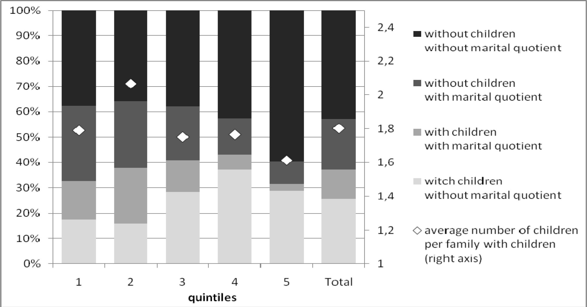

Distribution of household types and average number of children over the income distribution.
Table 5 provides an overview of the change in disposable equivalent income across quintiles. Even though the change of scenario is revenue neutral, the average net change in disposable income amounts to the positive value of €63. This is due to using the concept of equivalent income. Mainly larger families with children gain in the alternative scenario, resulting in higher disposable equivalent income for proportionally more individuals.
Change of disposable equivalent income, split for tax increase and equivalent Euro and in percentage of baseline disposable equivalent income.
| quintiles | disposable equivalent income | net change | tax increase | parental subsidy | ||||
|---|---|---|---|---|---|---|---|---|
| baseline | alternative | Δ | % | Δ | % | Δ | % | |
| 1 | 8,156 | 8,210 | 54 | 1.03 | 271 | 2.88 | 337 | 4.35 |
| 2 | 12,374 | 12,313 | -61 | -0.52 | 434 | 3.54 | 386 | 3.12 |
| 3 | 15,392 | 15,427 | 36 | 0.18 | 357 | 2.36 | 393 | 2.54 |
| 4 | 18,933 | 19,099 | 166 | 0.88 | 257 | 1.36 | 423 | 2.24 |
| 5 | 26,827 | 26,963 | 116 | 0.46 | 185 | 0.72 | 301 | 1.18 |
| Total | 16,336 | 16,402 | 62 | 0.41 | 301 | 2.17 | 368 | 2.69 |
-
Source: MISIM.
Overall, net changes are limited in all quintiles. On average, the parental subsidy is rather evenly distributed over the income distribution. Because of relatively fewer children in the extreme quintiles, the amount of the average parental subsidy is slightly smaller in these quintiles. The tax increase due to abolition of the marital quotient system is less evenly distributed: loss is largest in the second quintile, where the martial quotient is most frequent. Relative to disposable equivalent income in the baseline scenario, disposable income in the first quintile rises most strongly, because of the lower baseline equivalent income, followed by the fourth quintile, because of the highest concentration of children under 13 in this quintile. The second is the only quintile where the net change in disposable equivalent income is negative. This is due to the fact that families that make use of the marital quotient system are concentrated in quintile 2, and to a lesser extent in quintile 3, where the net change remains below average as well.
In Table 6, the division between gainers, losers and unaffected individuals is further investigated. A person is considered unaffected if his change in yearly disposable equivalent income from the baseline to the alternative scenario remains below €10. It is confirmed that gainers are situated mostly in the upper middle quintiles, while losing families are concentrated in the lower middle quintiles. Nevertheless, the 25% gaining households in the first quintile gain most of all quintiles, both in relative and in absolute numbers. The explanation is twofold. On the one hand, the families with children in the lower quintiles are slightly more numerous than on average (see Figure 1). on the other hand, the amount a household gains from using the marital quotient tends to rise with income, resulting in a smaller loss in the first quintile (at least in absolute numbers; in relative terms the households at the lower end of the income distribution that lose income face the largest decline in disposable income, expressed as a % of the income in the baseline scenario). Accordingly, for families in the first quintile with children that make use of the marital quotient, the average gain is least affected by the losses due to tax increase, resulting in a higher gain in absolute numbers.
Gainers and losers, average gain per gainer and average loss per loser, in equivalent Euros and in percentage of baseline disposable equivalent income.
| quintiles | % gainers | % losers | % unaffected | average gain/gainer in disp. eq. inc. | average loss / loser in disp. eq. inc. | ||
|---|---|---|---|---|---|---|---|
| Δ | % | Δ | % | ||||
| 1 | 26.20 | 31.97 | 41.84 | 910 | 11.51 | -577 | -6.22 |
| 2 | 29.62 | 41.87 | 28.52 | 823 | 6.64 | -727 | -5.93 |
| 3 | 35.55 | 41.12 | 23.33 | 809 | 5.21 | -612 | -4.06 |
| 4 | 40.31 | 33.33 | 26.36 | 870 | 4.62 | -555 | -2.95 |
| 5 | 30.13 | 24.70 | 45.17 | 823 | 3.24 | -535 | -2.09 |
| Total | 32.36 | 34.60 | 33.04 | 847 | 6.24 | -601 | -4.25 |
-
Source: MISIM.
For the second quintile, the average loss per loser is the highest of all quintiles in absolute disposable equivalent income. Not only contains the second quintile the highest share of marital quotient using families, the incomes of these families are substantial enough to lead to considerable advantages of using the marital quotient, as well as losses when it is abolished.
Table 7 presents a more detailed picture and reveals the profile of the gainers and losers. Households with children that do not make use of the marital quotient system are the main gainers in the alternative scenario. Households without children that make use of the marital quotient system are unanimously losers. The unaffected exceptions in the lower quintiles are most probably households whose allowance due to the marital quotient is too low – because of low income of both spouses – to result in a significant change in yearly disposable income. The average absolute amount that the families in this category lose rises with their income. This is a logical consequence of the system’s feature that the amount a household gains from using the marital quotient tends to rise with income. The progressivity of the Belgian tax system causes the marginal tax rate against which the income of the earning spouse would be taxed when it was not transferred to the other spouse to be higher for high income marital quotient users. In both relative and absolute terms, low income marital quotient users, as a consequence, benefit less from it than their high income counterparts, or lose less in the case of its abolition.
Gainers and losers, average gain per gainer and average loss per loser, in equivalent Euros and in percentage of disposable equivalent income, for the 4 family types.
| quintile s | With children and no MQ | With children and with MQ | No children and no MQ | No children and with MQ | ||||||||
|---|---|---|---|---|---|---|---|---|---|---|---|---|
| % gainer % losers % unaffected |
average gain/gainer or loss/loser | % gainer % losers % unaffected |
average gain/gainer or loss/loser | % gainer % losers % unaffected |
average gain/gainer or loss/loser | % gainer % losers % unaffected |
average gain/gainer or loss/loser | |||||
| Δ | % | Δ | % | Δ | % | Δ | % | |||||
| 1 | 97% | 1064 | 13.32 | 59% | 639 | 8.32 | 0% | 0 | 0.00 | 0% | 0 | 0.00 |
| 0% | 0 | 0.00 | 39% | -394 | -4.50 | 13% | -171 | -2.08 | 72% | -721 | -7.65 | |
| 2 | 3% | 0 | 0.00 | 2% | 0 | 0.00 | 87% | 0 | 0.00 | 28% | 0 | 0.00 |
| 97% | 890 | 7.19 | 65% | 749 | 6.04 | 0% | 0 | 0.00 | 0% | 0 | 0.00 | |
| 0% | 0 | 0.00 | 34% | -427 | -3.45 | 27% | -155 | -1.24 | 95% | -1033 | -8.45 | |
| 3 | 3% | 0 | 0.00 | 1% | 0 | 0.00 | 73% | 0 | 0.00 | 5% | 0 | 0.00 |
| 100% | 866 | 5.55 | 55% | 585 | 3.86 | 0% | 0 | 0.00 | 0% | 0 | 0.00 | |
| 0% | 0 | 0.00 | 45% | -536 | -3.62 | 39% | -126 | -0.82 | 99% | -977 | -6.47 | |
| 4 | 0% | 0 | 0.00 | 0% | 0 | 0.00 | 61% | 0 | 0.00 | 1% | 0 | 0.00 |
| 100% | 898 | 4.77 | 54% | 562 | 2.96 | 0% | 0 | 0.00 | 0% | 0 | 0.00 | |
| 0% | 0 | 0.00 | 46% | -562 | -2.92 | 39% | -133 | -0.70 | 98% | -1054 | -5.61 | |
| 5 | 0% | 0 | 0.00 | 0% | 0 | 0.00 | 61% | 0 | 0.00 | 2% | 0 | 0.00 |
| 100% | 831 | 3.28 | 44% | 600 | 2.07 | 0% | 0 | 0.00 | 0% | 0 | 0.00 | |
| 0% | 0 | 0.00 | 56% | -561 | -2.11 | 24% | -114 | -0.47 | 100% | -1,193 | -4.65 | |
| 0% | 0 | 0.00 | 0% | 0 | 0.00 | 76% | 0 | 0.00 | 0% | 0 | 0.00 | |
-
Source: MISIM.
The category of families without children and without using the marital quotient system remains least affected. The fact that there is a proportion of this category losing a modest amount despite not making use of the marital quotient is due to the transfer of personal tax allowance between partners (see Section 3.4).
Finally, the category of households with children that make use of the marital quotient system is the most heterogeneous group with respect to gains and losses. With the parental subsidy depending on the number and the age of the children, the assigned sums can vary substantially from household to household. For the majority of the households, the parental subsidy outweighs the tax increase. Still, for a considerable fraction of the households belonging to this type, the parental subsidy does not compensate for the loss due to the removal of the marital quotient system. This fraction grows over the quintiles, as the gains from marital quotient tend to increase with income. The families that lose are most probably families with fewer and older children.
Average net change in yearly disposable equivalent income and in percentage of baseline disposable equivalent income for various age groups.
| quintiles | 0 to 12 | 13 to 18 | 19 to 34 | 35 to 49 | 50 to 64 | 65 to 74 | 75+ | Total |
|---|---|---|---|---|---|---|---|---|
| 1 | 849 | -80 | 211 | -2 | -211 | -259 | -207 | 54 |
| 10.61 | -0.62 | 2.79 | 0.37 | -2.25 | -2.54 | -2.09 | 1.03 | |
| 2 | 750 | -1 38 | 1 39 | -33 | -469 | -500 | -355 | -61 |
| 6.05 | -1.13 | 1.11 | -0.30 | -3.83 | -4.07 | -2.92 | -0.52 | |
| 3 | 788 | -1 1 1 | 1 50 | 46 | -424 | -443 | -454 | 36 |
| 5.06 | -0.76 | 0.92 | 0.25 | -2.81 | -2.89 | -3.00 | 0.18 | |
| 4 | 880 | 76 | 196 | 204 | -437 | -324 | -377 | 1 66 |
| 4.69 | 0.44 | 1.02 | 1.10 | -2.32 | -1.75 | -2.02 | 0.88 | |
| 5 | 860 | 85 | 82 | 1 86 | -280 | -303 | -265 | 116 |
| 3.38 | 0.35 | 0.34 | 0.70 | -1.06 | -1.24 | -1.10 | 0.46 | |
| Total | 824 | -55 | 151 | 96 | -358 | -378 | -319 | 62 |
| 5.90 | -0.48 | 1.12 | 0.48 | -2.37 | -2.90 | -2.45 | 0.41 |
-
Source: MISIM.
Table 8 employs an intergenerational perspective. While the age categories of young children and parents gain across all quintiles, from the age of 50 onward one finds oneself worse off in the alternative scenario independent of one’s position in the income distribution. Inside each age category, the relative gains and losses tend to be more important at the bottom of the income distribution than at the top. Still, the gainer/loser- division of our proposed reform stands out very clearly as an intergenerational one.
4.3 Effect on poverty and inequality
The poverty figures are based on a poverty line parental subsidy creates between children under calculated as 60% of median equivalent income and children over 13 years of age. For the over the entire population, for the baseline and youngest children up to 3 years, poverty rates are the alternative scenario. We use a floating poverty being almost halved. For children aged 13 to 17, line, which remains however relatively stable between the different scenarios. In the baseline scenario, the poverty line lies at €9,116 of yearly disposable equivalent income, rising slightly to €9,162 in the alternative scenario.
Table 9 shows how poverty among children drops in the alternative scenario. This decrease, however, conceals the considerable gap the parental subsidy creates between children under and children over 13 years of age. For the youngest children up to 3 years, poverty rates are being almost halved. For children aged 13 to 17, the poverty rate slightly increases, yet not significantly. Poverty rates for the elderly increase as well, since elderly make up an important part of the main group that loses from the alternative measure, namely families using the marital quotient system without having young children leading to the parental subsidy.
Poverty rates with confidence intervals (*) by age group.
| Baseline | Alternative | ||||||||
|---|---|---|---|---|---|---|---|---|---|
| Categories | Population share | Poverty Rate | S.E. | C.I. (95%) | Poverty Rate | S.E. | C.I. (95%) | ||
| Overall | 100% | 11.71 | 0.68 | 10.37 | 13.05 | 12.19 | 0.65 | 10.90 | 13.47 |
| Children (0–17) | 22% | 10.08 | 1.05 | 8.01 | 12.16 | 8.60 | 0.94 | 6.75 | 10.45 |
| 0-3 | 4% | 12.22 | 1.90 | 8.47 | 15.97 | 7.10 | 1.49 | 4.16 | 10.03 |
| 4–12 | 12% | 7.99 | 0.96 | 6.10 | 9.88 | 5.97 | 0.80 | 4.40 | 7.54 |
| 13–17 | 6% | 12.66 | 1.74 | 9.24 | 16.08 | 14.50 | 1.80 | 10.96 | 18.05 |
| Adults (18–64) | 62% | 10.22 | 0.70 | 8.85 | 11.59 | 10.79 | 0.69 | 9.43 | 12.16 |
| Elderly (65+) | 16% | 19.94 | 1.27 | 17.43 | 22.45 | 22.74 | 1.38 | 20.02 | 25.47 |
-
Source: MISIM.
(*) Confidence intervals are based on a Taylor-linearized variance estimation (Greene, 2000).
Table 10 compares the change in poverty rates for the four family types. Poverty among families with children that do not use the marital quotient system falls, while poverty among families without children that do make use of the marital quotient system rises significantly. For families belonging to the other two categories, the figures remain more or less stable. On the one hand, the parental subsidy compensates the loss of the marital quotient system for the families with children that formerly made use of it, and on the other hand the system leaves families without children and without using the marital quotient system largely unaffected under the alternative scenario. The population shares of each group show the degree to which the marital quotient system is outdated. While some 30% of the population is making use of this allowance in the Belgian tax system, only 1/3 of this group lives in a family with children younger than 13. The larger part of the marital quotient using families has no young children (anymore). Moreover, of the current parents with young children, only a minority is making use of the marital quotient system, while most live in dual earner families or consist of single parent families.
Poverty rates with confidence intervals (*) for 4 family types by the presence of children and use of marital quotient system.
| Baseline | Alternative | ||||||||
|---|---|---|---|---|---|---|---|---|---|
| Categories | Population share | Poverty Rate | S.E. | C.I. (95%) | Poverty Rate | S.E. | C.I. (95%) | ||
| Overall | 100% | 11.71 | 0.68 | 10.37 | 13.05 | 12.19 | 0.65 | 10.90 | 13.47 |
| With children and no MQ | 26% | 7.02 | 0.95 | 5.15 | 8.89 | 4.25 | 0.73 | 2.83 | 5.68 |
| With children and with MQ | 12% | 13.61 | 1.97 | 9.73 | 17.50 | 13.37 | 2.05 | 9.33 | 17.41 |
| No children and no MQ | 43% | 11.60 | 0.75 | 10.12 | 13.07 | 11.70 | 0.76 | 10.22 | 13.19 |
| No children and with MQ | 20% | 16.82 | 1.30 | 14.27 | 19.37 | 22.61 | 1.42 | 19.81 | 25.42 |
-
Source: MISIM.
(*) Confidence intervals are based on a Taylor-linearized variance estimation.
Inequalit measures.
| Baseline | Alternative | |||||||
|---|---|---|---|---|---|---|---|---|
| S.E. | C.I. (95%) | S.E. | C.I. (95%) | |||||
| Gini | 0.2294 | 0.0032 | 0.2231 | 0.2356 | 0.2321 | 0.0031 | 0.2261 | 0.2381 |
| GE(-1) | 0.1684 | 0.0113 | 0.1462 | 0.1907 | 0.1695 | 0.0113 | 0.1475 | 0.1916 |
| MLD | 0.1014 | 0.0035 | 0.0946 | 0.1082 | 0.1029 | 0.0034 | 0.0963 | 0.1095 |
| Theil | 0.0887 | 0.0026 | 0.0836 | 0.0937 | 0.0902 | 0.0025 | 0.0853 | 0.0951 |
| GE(2) | 0.0918 | 0.0030 | 0.0860 | 0.0976 | 0.0934 | 0.0029 | 0.0876 | 0.0991 |
| GE(3) | 0.1076 | 0.0046 | 0.0986 | 0.1166 | 0.1093 | 0.0046 | 0.1003 | 0.1183 |
-
Source: MISIM.
-
*
Confidence intervals are based on a Taylor-linearized variance estimation.
A decomposition of these figures into within group and between group inequality (see Table 12) reveals a sharp increase in between-group inequality for both age groups and family types. As we have seen in Table 9, the gap in average income between children and elderly people has further increased due to our reform. As a result, between-group inequality increases with 20%. This pattern reveals a sizable intergenerational redistribution from the older to the younger generations. Likewise, between-group inequality for the family types we defined rises sharply as well. Families with children that do not use the marital quotient are often two earner couples with a relatively high income, which is further supplemented by the parental subsidy. Those without children and using the marital quotient are typically older people with relatively lower incomes.
Within group and between group inequality (MLD16) under baseline and alternative scenario for various age groups and family types.
| Categories | Baseline | Alternative | ||||
|---|---|---|---|---|---|---|
| Within | Between | Within | %Δ | Between | %Δ | |
| Overall | 0.1014 | 0.1028 | 1.36% | |||
| Age groups | 0.0968 | 0.00462 | 0.0973 | 0.50% | 0.00558 | 21.21% |
| Children (0-17) | 0.0702 | 0.0678 | -3.38% | |||
| 0-3 | 0.0796 | 0.0681 | -14.48% | |||
| 4-12 | 0.0664 | 0.0620 | -6.70% | |||
| 13-17 | 0.0678 | 0.0705 | 4.03% | |||
| Adults (18–64) | 0.1101 | 0.1117 | 1.51% | |||
| Elderly (65+) | 0.0827 | 0.0843 | 1.98% | |||
| Family types | 0.0949 | 0.00651 | 0.0932 | -1.78% | 0.00967 | 48.54% |
| With children and no MQ | 0.0670 | 0.0593 | -11.61% | |||
| With children and with MQ | 0.0545 | 0.0518 | -4.90% | |||
| No children and no MQ | 0.1316 | 0.1321 | 0.41% | |||
| No children and with MQ | 0.0758 | 0.0777 | 2.49% | |||
-
Source: MISIM.
5. Conclusion
We have started from the observation that the Belgian income tax system has some “anachronistic features” when it comes to the issue of reconciling work and the family. The marital quotient, which was intended to support the breadwinner model, is increasingly beneficial to households without children, as single-income couples are more and more concentrated among older cohorts. The marital quotient is also an oddity in a personal income tax system that is becoming increasingly individualised.
Hence, we have simulated the effects of an alternative policy, which explicitly takes account of parental care efforts. This alternative aims to be neutral with respect to the choice between market- and self-provided services. On the basis of time-use data we have calculated a socially grounded amount of childcare time, which will be compensated for through a parental childcare subsidy. Abolition of the marital quotient provided the resources for this subsidy, which is in the first instance a revenue neutral operation. We have not included behavioural effects in our simulation, which leaves scope for future research.
The introduction of our alternative scenario leads to a considerable intergenerational redistribution. The main losers are older cohorts, who are in the current system the main beneficiaries of the marital quotient and who will not gain from the parental subsidy as they do not have young children. Not surprisingly, poverty among this group increases. The main winners are families with young children, often double earner couples that do not (or hardly) use the marital quotient. This intergenerational redistribution and increased poverty among the elderly call for concern (especially as the elderly are already identified as a vulnerable group). In future research we will explore accompanying measures that limit these side-effects.
Footnotes
1.
Since the 2001 personal income tax reform all measures applicable for married couples have been extended to couples that are statutory cohabiting.
2.
3.
There is no monetary sanction for underproviding, but sociologists argue that society disposes of a whole set of sanctioning mechanisms to signal deviance from the norm.
4.
Ideally, we would have liked to have some actual socially-normative childcare time based on a questionnaire or a similar source. As this does not exist, we develop the concept of socially grounded childcare time as a second- best alternative.
5.
There is no obvious time constraint for men with non-working spouses. Feminist scholars pointed out, however, that male breadwinner behaviour is made feasible to some extent by the mostly unseen support by the homemaker. As such, male breadwinner behaviour does not provide us with a solid indication of a potential working time that can be generalized in a society where dual earnership has become dominant.
6.
Strictly speaking the generalisation of survey outcomes for the Flemish region to the whole of Belgium may introduce bias. Yet, collective agreements, labor law and social security regulations are all federal matters and hence there is no reason to expect discrepancies in the distribution of working hours between Flemish parents and their French speaking counterparts.
7.
We selected the median rather than the mean because the latter is likely to be biased upwards by a limited number of outliers.
8.
The actual number varies between economic sectors (36 to 38 hours a week, obviously not including commuting time).
9.
Strictly speaking there is no such thing as a Belgian schooling system, since language communities are responsible for the organisation of their educational system. Yet, legal norms regarding the minimum weekly school hours and the organisation of these hours over the week are the same between the communities (e.g. primary school: a minimum of 28 periods of 50 minutes with a morning break of 15 minutes and a lunch break of 1 hour and no class on Wednesday afternoon). We therefore assume that the survey data on the Flemish community is also representative of the practice in the French and German speaking parts of Belgium.
10.
We use rounded median values for ages where children are in non-compulsory preschool, a rounded average of 30 hours for all years in primary school and thereafter a rounded median which was adjusted in an ad hoc way for the ages of 13, 14 and 15 because the strong variation in median values cannot be explained by institutional elements of the Belgian schooling systems (in this table: the Flemish community system).
11.
Hereby making abstraction of the fact that in reality for some parents, work hours may well deviate from the standard school hours.
12.
Amounts in this article refer to the year for which the simulation is performed. Most recent amounts are reported in footnotes. In tax year 2010 the maximum amount is € 9,280.
13.
In 2006 this measure has been extended to all children younger than 13. Since the simulations however concern the tax year 2004, we chose to simulate the measure in its configuration of that time. The amount of € 11.20 applies for both tax years 2004 and 2010.
14.
€ 510 for tax year 2010.
15.
More details on the features of these tax policies with respect to childcare and their simulation are to be found in Appendix.
16.
The other general entropy inequality measures investigated (with £ = -1 ; 1 ; 2) led to comparable results, and are therefore not reported.
17.
In the FFCS we found an estimated daily unit cost of 26 € (predicted monthly amount divided by predicted daily units), which represents a weighted average of subsidised and nonsubsidised childcare services including additional costs as those mentioned above.
18.
The standard errors around the mean are 3.4 and 8.4 € respectively.
19.
A second order polynomial is included because the official tariff structure is progressive in household income.
20.
The usual weekly working hours (paid employment) of the mother and father proved not to add to the prediction. Neither did the age of the youngest and the oldest child, nor the type of family (couple versus single parent).
Simulating the Belgian Childcare Tax Reduction
A.1 The context: tax regulation and childcare tariffs for tax year 2004
The Belgian income tax system incorporates a tax reduction related to cash expenditures for childcare services. The income tax system has two options. The parents choose (per child):
either to have a lump-sum raise of the household non-taxable income with €480 (for every child younger than 3 at the end of the income year)
or to reduce the taxable income of the household with the out-of-pocket costs of the childcare service for the full amount (though with €11.20 per day per child as a maximum). This second option is possible for outlays made for children before they reached the age of 3. The measure was extended in 2006 to children up to 12 years of age, but since the simulations concern the tax year 2004, we chose to simulate the configuration of that time.
Childcare expenses depend on the type of childcare services used, yet in practice the dominance of the subsidised sector (two thirds of the childcare places) forces non-subsidised service providers to keep their prices close to the In the subsidised sector a daily unit price is determined according to yearly taxable income of the parents and care use is measured in fractions of the daily unit, with 40% for any use below 3 hours, 60% for care use between 3 and 5 hours, 100% for use between 6 and 12 hours and 160% for more than 12 hours of contiguous childcare. Depending on the parents’ income the daily unit price varies between €1.41 and €25.18, but many parents pay close to the maximum amount because the tariff structure is steeply progressive with a relatively low maximum. Moreover, the daily unit cost is complemented with additional costs relating to specific items like meals and diapers.17
A.2. Imputation procedure
In the SILC-database information is available about the number of hours different types of childcare services are used in a ‘normal’ week (for every child separately), but no indications are given about the outlays connected to this childcare use. Fortunately, the FFCS-database combines information on the use of childcare services with an indicator of childcare expenses. More precisely, the FFCS indicates per child whether there is regular use of childcare services (‘yes’/‘no’) in a ‘normal’ week and details the hours of actual service use in a specific week (outside of holiday periods). Regarding the outlays the FFCS contains a variable relating to the total household expenses on childcare in a ‘normal’ month.
As could be expected the incidence of various types of childcare services differs according to the source of information. The gap between the sources is relatively small if the two measures based on use (‘yes’/‘no’) are used. An example on centre-based care (creches) is given in the table below. Interestingly, the indicator based on time- use data gives higher incidence figures. This is the case for most types of child-care services and most likely relates to non-regular use and to use that is seen as minor in relation to the type mentioned under the other questions.
The use of centre-based childcare in Flanders: a comparison of sources.
| SILC (use/hours) | FFCS (use) | FFCS (hours) | |
|---|---|---|---|
| None | 95.0 % | 91.0% | 83.8 % |
| For one child | 4.5 % | 8.1% | 13.8 % |
| For two children | 0.3 % | 0.7% | 2.3 % |
| For three children | 0.3 % | 0.3% | 0.2 % |
| N | 684 | 1577 | 394 |
| Indicator of use is | Types of childcare | Types of childcare | Hours of effective |
| based on: | services used in a ‘normal’ week | services used in a ‘normal’ week | use in the observation week |
-
Notes: all figures refer to families with any children < 13 in the region of Flanders SILC data are from 2004, FFCS from the school year 2004–2005 Data are weighted to correct for selective non-response.
As a first step towards imputation of the childcare expenses, we harmonised the types of childcare services from both data sources towards the categories shown in the following table.
Types of childcare services used by Flemish families in a normal week.
| FFCS | SILC | |
|---|---|---|
| Centre based care (crèche) | 9.0% | 5.0% |
| Childminder | 11.79% | 8.8% |
| Centre based care before and after school hours (other than school) | 7.8% | 0.9% |
| School care outside of school hours | 17.6% | 17.6% |
| Informal (grandparents and other) | 30.2% | 21.8% |
| Internate | 0.3% | 0.3% |
| Childminder at home under activation programme (‘PWA’) | 2.8% | 0.2% |
| Number of observations | 1577 | 684 |
-
Notes: all figures refer to families with any children < 13 in the region of Flanders SILC data are from 2004, FFCS from the school year 2004–2005 Data are weighted to correct for selective non-response.
Secondly we obtained from the FFCS parameter estimates on determinants that are available in both the FFCS and SILC. We differentiate between families with pre-school children (the ‘heavy’ service users) and families with schoolchildren who rely only on care services outside of school hours. In line with the differences in their care use, the average observed childcare expenses of the groups differ considerably: €45 a month for families with only schoolchildren versus €172 for families with younger children.18
We obtained OLS-results that predict the actual outcomes of families with school attending children quite robustly (R2=61.6%), but obtaining strong results for the group of pre-school children proved more difficult (R2=41.4%). As predictors we use the household net monthly income,19 the number of children that are in a particular type of care in a normal week and the number of hours spent in a particular type of care in the observation week.20 With the parameter estimates we are able to simulate in the SILCdataset the monthly expenses for childcare.
Yet, tax deductions related to childcare do not cover the full amount of the parental expenses. Rather there is a daily maximum expense (€11.20), that is likely to be binding for parents with preschool children, but not for the others given the limited number of hours their children need care before or after school. Therefore we need to figure out how many care days families use and whether these are likely to represent expenses below or above €11.20.
From the FFCS-data we learn that most of the care services use is concentrated in full-day care. Among families with young children, 72% use only care concentrated in one or more complete days and an additional 24% combine full-day care with half-day care, jointly covering almost all families. Since full-day care is charged at 100% and halfday care at 60% and the average daily rate is estimated at €26, all these families are likely to pass the daily limit of €11.20.
Therefore, we will not take the full amount of predicted childcare expenses into account for tax deductions, but determine the maximum deductible amount on the basis of the number of daily care units multiplied by €11.20. To do so in the SILC, we derive from the FFCS conversion estimates between the weekly hours of childcare use and the daily care units (OLS with R2 94.9%).
In the FFCS 81.6% of the families with young children proved to surpass with their (estimated) childcare expenses the (estimated) tax deductible amount and, hence, their childcare expenses were only taken into account up to the latter limit. In the calculations based on the SILC data, their share amounts to 86%.
References
-
1
Household production, full consumption and the costs of childrenLabour Economics 8:621–648.
-
2
A treatise on the family, enlarged editionCambridge MA/London: Harvard University Press.
- 3
-
4
Progressivity of Childcare Tax Policies in BelgiumLouvain Economic Review 74:143–165.
- 5
- 6
-
7
Time use in child care and housework and the total cost of childrenJournal of Population Economics 7:287–306.
-
8
The allocation and value of time assigned to housework and child-care: an analysis for SwitzerlandJournal of Population Economics 14:599–618.
-
9
An Inquiry into the Redistributive Effect of Personal Income Taxes in Belgium254, An Inquiry into the Redistributive Effect of Personal Income Taxes in Belgium, Ph.D. Thesis, Antwerp, UFSIA.
- 10
Article and author information
Author details
Acknowledgements
This article has been presented at the Second General Conference of the International Microsimulation Association in Ottawa, June 8th to 10th, 2009. We would like to thank participants of the conference, as well as two anonymous referees for helpful comments and suggestions.
Publication history
- Version of Record published: August 31, 2011 (version 1)
Copyright
© 2011, Ghysels
This article is distributed under the terms of the Creative Commons Attribution License, which permits unrestricted use and redistribution provided that the original author and source are credited.