A more efficient sampling procedure, using loaded probabilities
- JR Cumpston Pty Ltd, Australia
- Article
- Figures and data
-
Jump to
- Abstract
- 1. Introduction
- 2. Theory
- 3. Tests on accuracy
- 4. Example of the use of pools in simulating deaths
- 5. Run times with an australian microsimulation model
- 6. Checks on projected event numbers
- 7. Checks on event number standard deviations
- 8. Computational aspects
- 9. Likely applications
- 10. Conclusions
- References
- Article and author information
Abstract
All-case simulation, where demographic outcomes are simulated for each person each simulation cycle, has been used in almost every national household microsimulation model. This paper suggests the use of simulation by stratified sampling with loaded probabilities. This suggestion is intended to provide faster simulations, particularly when using simulation cycle times much shorter than a year. The paper derives optimal formulas for draw numbers and loaded probabilities, and uses stochastic simulations to show that sampling with loaded probabilities gives similar results to all-case simulation. Tests with a microsimulation model of 175,000 Australians show that sampling with loaded probabilities can reduce run times with yearly cycles by about 43%, and run times with weekly cycles by about 98%. A 50-year demographic projection took 34 seconds with a yearly cycle, and 54 seconds with a weekly cycle. Event numbers and standard deviations are comparable with those expected from risk profiles. The paper concludes that sampling with loaded probabilities is theoretically valid, can be much quicker than all-case simulation, and does give similar estimates. Potential applications are for large models, or those with short simulation cycles.
1. Introduction
1.1 All-case simulations
The first household microsimulation model developed in response to Orcutt’s 1957 proposals simulated demographic outcomes for each person in turn, working in the order in which the persons were stored (Orcutt, Greenberger, Korbel & Rivlin 1961). Unfortunately, processing persons in the same fixed order each cycle has the potential to introduce bias in some applications. Morrison (2006, p. 13) described the “sidewalk shuffle” alignment method, where persons in an alignment pool were sorted into random order before event simulation. Demographic outcomes were then simulated for the persons in the sorted pool, until the desired event total was reached. As the event probabilities were unchanged, the number of persons tested for the event was approximately equal to the number of persons in the pool.
1.2 Simulation by sampling with loaded probabilities
Testing every person for the occurrence of a demographic event seems inefficient, particularly for low-probability events. This paper proposes an alternative. Can we divide persons into pools, and only test a small proportion of persons in those pools with low probabilities? To ensure the correct expected number of events is still simulated, this partial sampling would be offset by loading the assumed probabilities of the event occurring. Such a process might be particularly efficient in short simulation cycles, where the probabilities of events occurring in the cycle are very low.
1.3 Structure of paper
The structure of the remainder of this paper is as follows. First, the theory under-pinning sampling with loaded probabilities is derived (Section 2). Tests on some simple cases with only two risk groups support the theory (Section 3). The large reductions in sample numbers feasible when simulating deaths are illustrated in Section 4, and Section 5 examines the actual run time reductions obtained in a realistic model. Section 6 compares expected and observed event numbers, for different simulation methods, cycle times and event orders. Section 7 similarly compares expected and observed event number standard deviations. Section 8 discusses computational aspects associated with implementation of this approach. Finally, Section 9 summarises the key findings from the paper, and considers in which situations use of simulation with loaded probabilities might be most appropriate.
2. Theory
2.1 A trivial case: Uniform event probabilities
Suppose we have 100 persons in a pool, each with 20% chance of death. To simulate the expected 20 deaths, we can randomly select any 20 persons from the pool, and declare them to have died. This simple procedure will rarely be applicable, as the expected number of events from a pool is unlikely to be an integer. For example, if there are 101 persons in the pool, each with a 20% chance of dying, then 20.2 deaths are expected. To obtain simulations with the correct expected number of deaths, we can randomly draw 21 persons from the pool, select a random number between 0 and 1 for each of them, and declare them to be dead if the random number is less than 20.2/21 (ie 0.9619). The number of draws needed in this case is reduced by 79%, increasing computational efficiency.
More formally, if there are n persons in a pool, each with probability pi of an event occurring, then the number of draws d needed from the pool is
Let qi be the loaded probability of the event occurring for each of the drawn persons.
Then
Substituting pi = 0.2, n = 101 and d = 21 gives qi = 0.9619, as above.
As each person has the same probability of the event occurring, this procedure works for events such as death where a person is lost from the pool, or events such as moves where the person remains within the pool.
2.2 Non-uniform event probabilities, with no losses from pool
The previous section assumed uniform probabilities. If persons in the pool have varying probabilities of the event occurring, a more complex loaded sampling procedure is needed. Suppose that the highest probability is pmax. From equation 2, restricting the maximum loaded probability to not exceed 1 requires that
so that the number of draws needed from the pool is
As before, the loaded probability of the event occurring for person i is given by equation 2. This analysis is appropriate for events not causing losses from a pool – for example, movements within a geographic pool.
2.3 Non-uniform event probabilities, with losses from pool
The previous section assumed no losses form the pool, but some events, such as deaths and emigration, will cause losses. As sampling proceeds from the pool, the cases most at risk are likely to be selected, and the risk profile within the pool will change. This requires some modifications to the formulas for loaded probabilities and draw numbers.
Let nt be the number of persons in the pool immediately before the tth draw (so that n1 = n). Also let qit be the loaded probability for person i during the tth draw. The probability of any person being picked in the tth draw is 1 / nt, so the probability of person i being simulated to have the event in draw t is qit / nt. The probability of person i not being simulated to have the event in any of d draws is
We do not know n2, n3 ... nd in advance, because they will depend on whether the preceding draws have removed any persons from the pool. But we can make the probability of person i being selected to have the event equal in each draw, by calculating loaded probabilities for each draw after the first with the formula
Substituting equation (6) in (5), and setting the result equal to the desired probability of person i not having the event, gives
Taking the 1/dth power of both sides and rearranging gives
Now qi1 is the loaded probability of person i being selected for the event in draw 1, and we do not want this to exceed unity. Thus we require, for all the persons in the pool, that
Taking logs of both sides and rearranging gives the requirement that
This can be achieved by taking d as
where pmax is the highest probability of the event occurring for any member of the pool. Note that if pmax is small and n large, this formula for d approximates to that in equation 4. Once d has been chosen using equation 12, it remains unchanged till all the d draws are completed. For the person selected for testing in the tth draw, the loaded probability qit can be calculated by combining equations 6 and 8 to get
As the number nt in the pool cannot increase above its initial value, the loaded probabilities cannot exceed their values for the first draw, and thus cannot exceed 1.
Table 1 shows the numbers of draws needed for pools of varying size, calculated using equation 12. The minimum number of draws from any pool is 1, so that sampling from very small pools becomes inefficient. If the maximum event probability for a pool is about 0.63 or higher, the number of draws will exceed the number of persons in the pool. In practice this is likely to occur for relatively few pools, a point illustrated in Section 4.
Number of draws to give maximum loaded probability of 1.
| Number in pool | maximum | unloaded | probability | |||
|---|---|---|---|---|---|---|
| 0.01 | 0.02 | 0.05 | 0.1 | 0.2 | 0.5 | |
| 10 | 1 | 1 | 1 | 2 | 3 | 7 |
| 100 | 2 | 3 | 6 | 11 | 23 | 69 |
| 1,000 | 11 | 21 | 52 | 106 | 224 | 693 |
| 10,000 | 101 | 203 | 513 | 1,054 | 2,232 | 6,932 |
| 100,000 | 1,006 | 2,021 | 5,130 | 10,536 | 22,315 | 69,315 |
2.4 Sampling with loaded probabilities with short simulation cycles
None of the above formulas depend on the length of the simulation cycle. The assumed probabilities of event occurrence are likely to have been based on annual simulation cycles, and will have to be appropriately recalculated for use with shorter simulation cycles.
2.5 Sampling with loaded probabilities with alignment
Sampling with loaded probabilities can be adapted to give event numbers conforming with external alignment totals
The highest probability of the event occurring in the alignment pool, or some upper limit to that probability, is assumed to be known
An individual is randomly selected from the pool, their probability divided by the highest probability, and a random number drawn to see if the event occurs
The process is repeated until the desired alignment total is reached.
This process is similar to the sidewalk shuffle described by Morrison (2006), except that random shuffling of the persons in the pool is replaced by repeated random selection.
2.6 Uses of simulation by sampling with loaded probabilities in other fields
Given its generality, it is likely that similar processes are being used for applications in other fields. Sampling with loaded probabilities uses stratified sampling (Ross 2006: 66–184), one of a wide range of variance reduction techniques used in simulation.
3. Tests on accuracy
There was some concern that the formulas in Section 2.3 might not give completely correct results in practice. To test this, 10,000 repeated trials were made with risk pools containing varying numbers of low risk cases, and 500 high risk cases. In the first set of trials, 2,500 low-risk cases were assumed, each with probability of 0.1, so that 250 events were expected from the low-risk cases. In the second to fifth set of trials, the assumed probability for the low-risk cases was progressively increased, and their number reduced, so as to maintain the expected number of low-risk events at 250. In each set of trials, the 500 high-risk cases were assumed to have probability 0.5, so that 250 events were expected from them. In each set of trials, 500 events were thus expected.
Table 2 shows that the mean numbers of simulated events were all very close to the expected 500. The worst deviation from the expected 500 events was 0.12, for the second and third set or trials. In no case was the deviation from the expected 500 events greater than the standard deviations in the last column of Table 2. These standard deviations are the standard deviations in the observed event numbers from 10,000 trials, divided by 100 (the square root of the number of trials). These results suggest that sampling by loaded probabilities, for the case with non-uniform event probabilities and losses from the pool, can work correctly.
Simulated event numbers with pools chosen to produce 500 events.
| Number low risk persons | Low risk rate | Number high risk persons | High risk rate | Expected number of events | Mean number from 10,000 trials | Standard deviation from 10,000 trials |
|---|---|---|---|---|---|---|
| 2,500 | 0.1 | 500 | 0.5 | 500 | 499.92 | .16 |
| 1,250 | 0.2 | 500 | 0.5 | 500 | 500.12 | .14 |
| 833 | 0.3 | 500 | 0.5 | 500 | 499.88 | .12 |
| 625 | 0.4 | 500 | 0.5 | 500 | 500.03 | .10 |
| 500 | 0.5 | 500 | 0.5 | 500 | 500.00 | .09 |
4. Example of the use of pools in simulating deaths
In practice, there can be considerable heterogeneity in risk rates, so that segregation into a small number of risk groups can greatly reduce the numbers of draws needed to simulate the expected numbers of events. This is illustrated in Table 3, using Australian data on ages and mortality rates.
Table Draws needed to simulate the deaths in a year 175,000 Australians.
| Age group | Persons in group | Average mortality rate | Expected deaths | Maximum mortality rate | Draws |
|---|---|---|---|---|---|
| 0- | 36,441 | 0.00040 | 14.5 | 0.00453 | 166 |
| 15- | 23,593 | 0.00060 | 14.1 | 0.00113 | 27 |
| 25- | 25,575 | 0.00087 | 22.1 | 0.00138 | 36 |
| 35- | 26,810 | 0.00123 | 33.0 | 0.00192 | 52 |
| 45- | 24,156 | 0.00237 | 57.2 | 0.00415 | 101 |
| 55- | 16,348 | 0.00642 | 104.9 | 0.01315 | 217 |
| 65- | 11,852 | 0.01826 | 216.4 | 0.03697 | 447 |
| 75- | 7,706 | 0.05051 | 389.3 | 0.10627 | 866 |
| 85- | 2,563 | 0.18238 | 467.4 | 0.48496 | 1701 |
| Total | 175,044 | 0.00754 | 1,319.0 | 3,613 |
The numbers of expected deaths in Table 3 were estimated by applying 2001-02 mortality rates to a sample of 175,044 persons derived from the 1% 2001 census sample file. The maximum mortality rates are the highest applying to any age in each of the groups. For example, the highest mortality rate for the 0–14 group is for males aged 0, while the highest rate for persons 85+ is for females aged 110. The numbers of draws needed with loaded sampling were calculated from equation 12. For example, the number of draws needed from the pool for persons 55-64 was calculated as
These estimates suggest that good simulations of the deaths in a year can be made by 3,613 draws with loaded probabilities, rather than 175,044 draws with true mortality rates. Note that, for this empirical example, the identified pmax of 0.485 for the highest-risk group is less than 0.63 – the tipping point at which the number of draws starts to exceed the number of persons in the pool.
5. Run times with an australian microsimulation model
5.1 Pools used to test sampling with loaded probabilities
In order to explore the achievable efficiency gains offered by sampling with loaded probabilities, the technique was applied to a dynamic microsimulation model of Australia. The pools in this model used here are each combination of 8 areas, 8 person types and 9 age groups (see Table 4), making 576 pools in all.
Areas, person types and age groups used to form pools.
| Area code | Area name | Person type code | Person type | Age code | Age group |
|---|---|---|---|---|---|
| 1 | NSW | 1 | Partner | 1 | 0–14 |
| 2 | Victoria | 2 | Lone parent | 2 | 15–24 |
| 3 | Queensland | 3 | Child | 3 | 25–34 |
| 4 | SA | 4 | Related person | 4 | 35–44 |
| 5 | WA | 5 | Unrelated person | 5 | 45–54 |
| 6 | Tasmania | 6 | Lone person | 6 | 55–54 |
| 7 | NT | 7 | Group member | 7 | 65–74 |
| 8 | ACT | 8 | Non-private resident | 8 | 75–84 |
| 9 | 85- |
These pools were available for alignment purposes, and not specifically chosen for sampling with loaded probabilities. With hindsight, these pools were too fine for sampling with loaded probabilities, and resulted in simulated numbers of exits and moves being a little different from expected. These errors, and ways to minimize them, are discussed in Section 6.1.
5.2 Run times to simulate 175,000 Australian for a year
The run times in Table 5 exclude the input of data and assumptions before a run, and the time needed to output results. Maximum probabilities for each risk group are included in the assumptions file, which takes about 0.3 seconds to read. There were some unexpectedly large random variations in run times for the first cycle, so all the run times with yearly cycles are the average of 50 runs. All the multi-cycle all-case run times are from single runs, and all the multi-cycle loaded run times are the averages of at least 3 runs.
Mean run times in seconds to simulate 175,000 Australians for a year.
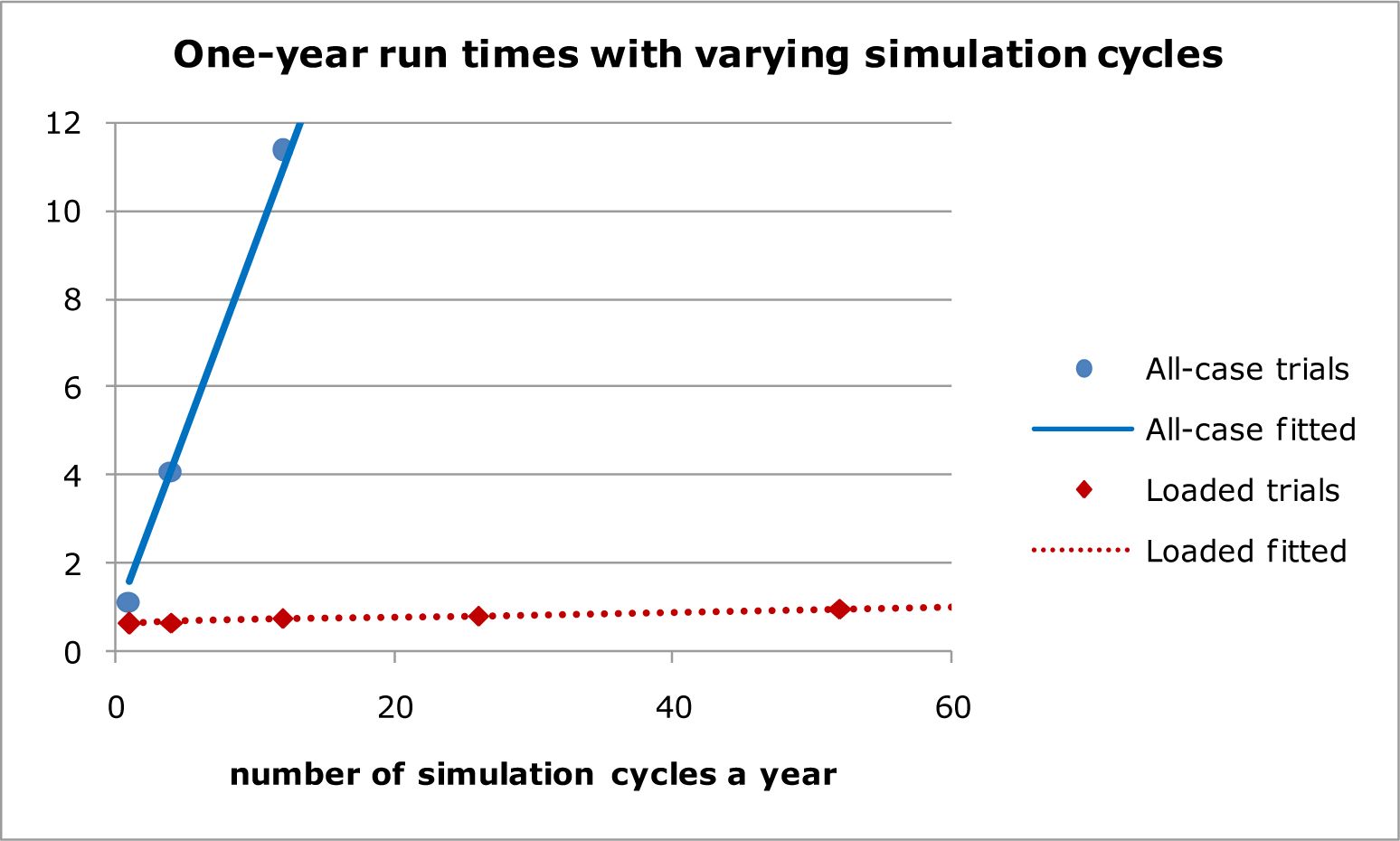
| Cycles per year | All-case trials seconds | All-case fitted seconds | Loaded trials seconds | Loaded fitted seconds | Loaded trials as % of all-case |
|---|---|---|---|---|---|
| 1 | 1.13 | 1.58 | 0.64 | 0.66 | 57% |
| 4 | 4.10 | 4.14 | 0.67 | 0.68 | 16% |
| 12 | 11.37 | 10.98 | 0.75 | 0.73 | 7% |
| 26 | 23.29 | 22.94 | 0.83 | 0.82 | 4% |
| 52 | 44.90 | 45.15 | 0.98 | 0.97 | 2% |
| 365 | 2.88 | 2.88 |
The run times in Table 5 exclude the input of data and assumptions before a run, and the time needed to output results. Maximum probabilities for each risk group are included in the assumptions file, which takes about 0.3 seconds to read. There were some unexpectedly large random variations in run times for the first cycle, so all the run times with yearly cycles are the average of 50 runs. All the multi-cycle all-case run times are from single runs, and all the multi-cycle loaded run times are the averages of at least 3 runs.
Table 5 shows that the times required with all-case simulations increase broadly in line with the number of cycles a year. The slope and constant obtained by fitting a linear trend line by least squares minimization suggest that sampling each case takes about 0.85 seconds a cycle, and adjusting data in response to simulated events takes about 0.72 seconds a year, with a poor fit for yearly cycles (see Table 5). The slope and constant from the trend-line fit with loaded probabilities suggest that sampling takes about 0.006 seconds a cycle, and adjusting data in response to simulated events takes about 0.66 seconds a year. The fit with loaded probabilities is good up to 365 cycles a year. The numbers of simulated events, and the time taken to process them, should be very similar with both methods. As expected, the time savings are in sampling.
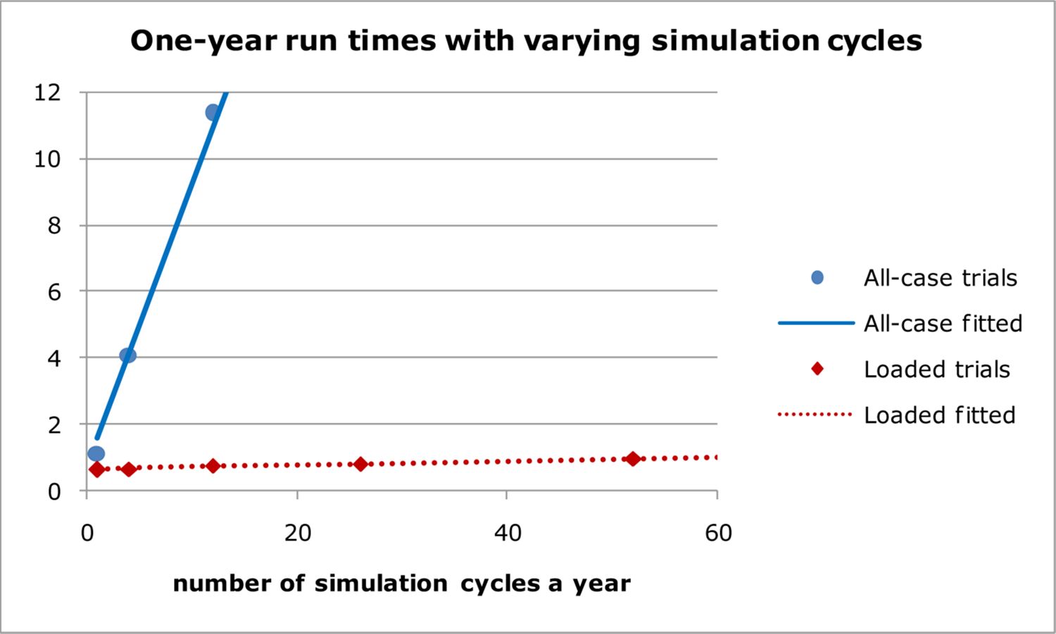
Run times with varying simulation cycles.
5.3 Run times for projections for up to 50 years
The yearly values in the first line of Table 6 are those in the first line of Table 5. They show sampling with loading probability has a one-year run-time about 57% of all-case sampling, which is out of line with the 53% or 52% in the multi-year lines of Table 6. Comparing the calculation steps involved in all-case and loaded sampling suggests that the savings from loaded sampling should be a constant proportion, regardless of the number of projection years. The one-year result is an anomaly.
Run times in seconds for projections up to 50 years.
| Projection years | All-case Yearly | Loaded Yearly | Loaded Weekly | Loaded as% of all case Yearly |
|---|---|---|---|---|
| 1 | 1.13 | 0.64 | 0.98 | 57% |
| 10 | 11.59 | 6.18 | 9.81 | 53% |
| 20 | 24.28 | 12.82 | 20.28 | 53% |
| 30 | 37.35 | 19.72 | 31.2 | 53% |
| 40 | 51.93 | 27.25 | 42.51 | 52% |
| 50 | 66.32 | 34.16 | 53.87 | 52% |
Figure 2 shows that both all-case and loaded sampling methods have a slight increase in run time per year for higher projection times. This is because of the population growth of about 30% projected over the 50 years.
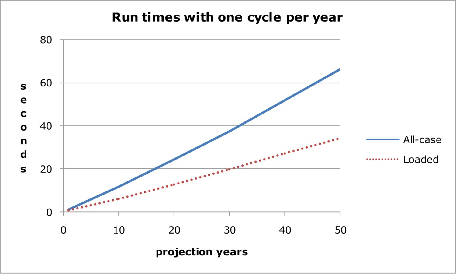
Run times with one cycle per year.
6. Checks on projected event numbers
This section compares the expected numbers of each type of movement, with the average numbers observed with different cycle time, sampling methods and event orders. The types of event examined are births, deaths, emigrants, exits and moves. Immigrants were not compared, because the microsimulation model pregenerates immigrant families to match exogenous immigrant assumptions. An “exit” is a departure from a household of a person, possibly followed by one or more of the other household members. By contrast, a “move” is where the whole household moves to another dwelling. For various reasons, the observed numbers differ from expected by more than can be explained by random variation. Nevertheless, the comparisons show that broadly reasonable results are being obtained.
6.1 One-year projection results with each event simulated separately
Table 7 shows the average numbers of projected events from 50 one-year runs, using either all-scase simulation or sampling with loaded probabilities. To avoid event interactions confusing the results, only one type of event was simulated in each run. Also shown are the expected numbers of events, obtained by summing the probabilities of each person having that event.
Event totals from one-year projections, each event simulated separately (50 run averages).
| Event | Expected | Observed all-case yearly | Observed loaded yearly | Observed loaded weekly |
|---|---|---|---|---|
| Births | 2,170 | 2,179 | 2,183 | 2,208 |
| Deaths | 1,372 | 1,379 | 1,330 | 1,370 |
| Emigrants | 2,284 | 2,280 | 2,251 | 2,275 |
| Exits | 6,254 | 6,441 | 6,203 | 6,592 |
| Moves | 12,468 | 12,411 | 12,330 | 12,364 |
Some of the possible reasons for the differences in Table 7 are:
Random variations in the numbers of simulated events. For example, if the expected 2,208 deaths were Poisson distributed, they would have a standard deviation of 47, and averaging over 50 runs would reduce this to about 7. The observed death numbers from all-case yearly and loaded weekly are thus within one standard deviation, while those from loaded yearly runs are well outside.
Derivation of the expected numbers in a manner inconsistent with the simulations. Event probabilities, particularly for births, exits and moves, depend on a number of person and household characteristics. While the expected probabilities for each person were based as closely as possible on the data at the start of the first projection year, some approximations may have occurred. One error in expected numbers was found during checking.
Movements between sampling pools resulting from births, deaths or emigrants. For example, if a partnered male is simulated to die, then his partner will be removed from a partner pool, and put into a pool of lone persons or lone parents. As deaths from these pools are simulated after deaths from partner pools, then the former partner may be double exposed to the risk of death. As birth, death and emigration are low-probability events, and some offsetting may occur, the resulting errors are likely to be small. A solution is to use pools based only on age.
Changes in type or area for exits. In the simulations with loaded probabilities, it was assumed that exits do not cause any losses from the pool. Trials show that about 86% of exits involve a type change, and about 10% involve an area change. With the area/type/age pool structure being used, changes of either type or area result in removal from the pool being simulated. This is not a problem with all-case simulations, but can cause insufficient persons to be sampled when using loaded probabilities. This seems likely to be a major reason why exits with a yearly cycle and loaded probabilities were 3.7% below the all-case number. A solution is to use pools based only on age, so that no pool losses occur.
Changes in area for moves. About 14% of moves involve an area change, and moves with a yearly cycle and loaded probabilities were 0.7% below the all-case number. Again, a solution is to use pools based only on age.
Changes in person types during the year. If type change assumptions are inappropriate, then there can be rapid changes in the numbers of particular types of persons in the first projection year. This may be a major reason for the 6% increase in exit estimates with loaded probabilities when changing from annual to weekly cycles.
Programming errors. The household microsimulation model used here was primarily constructed as a test-bed for different simulation techniques. It has been substantially validated and debugged, but there is potential for errors of the order of 10% in exit and move numbers to be still undetected, and for smaller errors in births, deaths and emigrants.
6.2 One-year projection results with all events simulated together
Table 8 shows the same expected numbers as Table 7, but with observed numbers obtained by simulating all events together. Within each simulation cycle, events have been simulated in the order births, deaths, emigrants, immigrants, exits and moves. Apart from moves, simulated event numbers are similar for both tables. Move numbers increased by about 8% for all-case simulation, 7% for loaded probabilities with a yearly cycle, and 4% for loaded probabilities with a weekly cycle. Move probabilities depend strongly on person types, so that poorly chosen exit assumptions can cause significant changes to moves in a year.
Event totals from one-year projections, all events simulated together.
| Event | Expected | Observed all-case yearly | Observed loaded yearly | Observed loaded weekly |
|---|---|---|---|---|
| Births | 2,170 | 2,175 | 2,182 | 2,232 |
| Deaths | 1,372 | 1,375 | 1,335 | 1,375 |
| Emigrants | 2,284 | 2,282 | 2,263 | 2,304 |
| Exits | 6,254 | 6,333 | 6,075 | 6,611 |
| Moves | 12,468 | 13,418 | 13,210 | 12,826 |
6.3 Comparisons between normal and reverse order simulations
Galler (1997) recommended short simulation cycles. To test their usefulness, simulations were made in normal and reverse order with yearly cycles, and then in normal and reverse order with weekly cycles.
Table 9 shows the changes from simulating events in reverse order are much smaller with weekly simulation cycles, particularly for exits and moves.
Table one-year projections, with events in normal & reverse order (50 run averages).
| Event | Yearly | Weekly | ||||
|---|---|---|---|---|---|---|
| normal order | reverse order | change in year | normal order | reverse order | change in year | |
| Births | 2,182 | 2,243 | 61 | 2,232 | 2,224 | -8 |
| Deaths | 1,335 | 1,331 | -4 | 1,375 | 1,378 | 3 |
| Emigrants | 2,263 | 2,308 | 45 | 2,304 | 2,311 | 7 |
| Exits | 6,075 | 6,540 | 465 | 6,611 | 6,615 | 4 |
| Moves | 13,210 | 12,323 | -887 | 12,826 | 12,819 | -7 |
These results strongly confirm the desirability of short simulation cycles.
6.4 Comparisons between all-case and loaded 50-year projections
Table 10 compares the averages of 10 50-year runs using all-case simulation with the averages of 10 runs using loaded probabilities. The expected numbers of births, deaths and emigrants are reasonably similar for both simulation methods. The 2.3% reduction in exits is less than the 4.1% for the one-year projections in Table 7, and may similarly reflect the assumption of no losses when most exits did in fact result in losses from the sampling pools. The 2.4% reduction in moves is more than the 0.7% in Table 7, and may reflect the 50-year accumulation of type errors when using loaded probabilities. Exits and moves do not affect person numbers, and the projected numbers of persons are very close.
50-year projections with yearly cycles (10 run averages).
| Event/persons at end | All-case yearly mean | All-case yearly SD | Loaded yearly mean | Loaded yearly SD | Loaded as % of all-case |
|---|---|---|---|---|---|
| Births | 102,831 | 541 | 101,611 | 516 | 98.8% |
| Deaths | 92,205 | 127 | 91,924 | 130 | 99.7% |
| Emigrants | 123,775 | 186 | 123,024 | 232 | 99.4% |
| Exits | 355,304 | 891 | 347,052 | 746 | 97.7% |
| Moves | 797,511 | 1,716 | 778,254 | 937 | 97.6% |
| Persons at end | 226,755 | 488 | 226,566 | 504 | 99.9% |
7. Checks on event number standard deviations
From initial trials, it was noted that simulations with loaded probabilities sometimes gave much lower standard deviations in event numbers than all-case simulations. This was unexpected, but investigation showed that low standard deviations were likely when sampling from pools with limited probability ranges. Some approximate theoretical estimates of expected standard deviations were thus made, and compared with the observed standard deviations with the two methods with a yearly cycle, and with loaded probabilities with a weekly cycle.
Table 11 compares approximate expected standard deviations for each event type with those observed from 50 runs, simulating all events together. For each sampling pool, the average loaded probability was calculated as
Standard deviations for one-year projections (based on 50 runs).
| Event | All-case Yearly | All-case Yearly | Loaded Yearly | Loaded Yearly | Loaded weekly | Loaded weekly |
|---|---|---|---|---|---|---|
| Expected | Observed | Expected | Observed | Expected | Observed | |
| Births | 43.8 | 38.6 | 43.6 | 38.7 | 43.5 | 52.8 |
| Deaths | 35.4 | 32.7 | 28.0 | 29.9 | 31.7 | 32.2 |
| Emigrants | 47.3 | 38.6 | 26.2 | 35.6 | 36.5 | 42.8 |
| Exits | 73.7 | 67.6 | 33.2 | 39.8 | 54.7 | 59.6 |
| Moves | 98.3 | 99.7 | 10.3 | 18.9 | 50.0 | 55.1 |
where the number of draws was calculated using equation 4 or 12.
The expected variance of the number of events from that pool was then approximately estimated assuming the variance formula for a binomial distribution
Variances were summed across all pools, and the square root taken to give an approximate estimate of the standard deviation. Given the approximate nature of the expected standard deviations, and the broad confidence limits generally associated with standard deviation observations, the expected and observed standard deviations are reasonably comparable.
As shown in Table 2, sampling with loaded probabilities can give low standard deviations, particularly for risk combinations with a narrow range of risks. This is because the loaded probabilities can all be close to 1, and there will be little variability in the simulated numbers of events. For moves, most of the persons in each sampling pool had similar probabilities, so that loaded probabilities with a one-year simulation cycle gave standard deviations that were much lower than with all-case sampling.
As the number of simulation cycles in a year increases, more pools have very low numbers of expected events, with loaded probabilities well below 1, and higher variability in simulated numbers of events. Comparing the values for loaded simulations with yearly and weekly cycles, all the observed standard deviations increased, and particularly so for moves.
The coefficients of variation in Table 12 were obtained by dividing the observed standard deviations in Table 11 by the observed numbers in Table 8. Regardless of simulation method or cycle length, the coefficients of variation for the tested model are small, and may not be important in most practical applications.
Observed coefficients of variation for one-year projections (based on 50 runs).
| Event | All-case Yearly | Loaded yearly | Loaded weekly |
|---|---|---|---|
| Births | 0.018 | 0.018 | 0.024 |
| Deaths | 0.024 | 0.022 | 0.023 |
| Emigrants | 0.017 | *0.016 | 0.019 |
| Exits | 0.011 | 0.007 | 0.009 |
| Moves | 0.007 | 0.001 | 0.004 |
8. Computational aspects
Computational details for loaded sampling will depend strongly on the database structure and programming language. Test results here are from a model using a list structure rather than a relational database. A separate list is maintained of member addresses for each of 576 pools (each combination of 8 areas, 8 person types and 9 age groups). These pools are maintained for alignment purposes, but they also proved useful for loaded sampling. All data for a person are stored as a single line in an array, and their address in the array is recorded in the relevant pool list. The address of each new person in a pool is added to the end of the list. The address of any exiting person is replaced in the list by the address currently at the end of the list, with the length of the list being reduced by one. A random number is drawn, and multiplied by the length of the list, to randomly select a person from a pool
A similar list structure has been used by INHASIM for many years (Inagaki 2009). INHASIM uses a template class of sequence containers, based on Microsoft’s Visual C++ STL list class, that maintains its elements in a linear arrangement and allows efficient insertions and deletions at any location within a sequence.
9. Likely applications
In practice, where is sampling with loaded probabilities likely to be useful? Models with fine geographic subdivisions will generally require at least 1,000 persons to realistically represent each subdivision, and may thus become very large. Models with many different types of physical disability will also need to be large, so as to adequately represent uncommon disabilities. Models including processes with short time spans are also likely to get useful time savings from sampling with loaded probabilities. For example, a microsimulation model of dwelling sales and rentals is likely to need both a detailed geographic structure, and a simulation cycle of a week or less.
Existing models of moderate size but unusually slow run times are unlikely to benefit from sampling with loaded probabilities. Their slowness may reflect programming and data storage issues, or excessive use of alignment, and more efficient sampling will have little effect. Adding sampling with loaded probabilities to any existing model may require changes to data indexing procedures, and will require additional model validation.
Fredriksen, Knudsen & Stolen (2011) describe the use of multithreading to greatly reduce runtimes in the MOSART model of the whole Norwegian population. They comment that simulation steps involved in household formation are cumbersome to multi-thread, due to often subtle interactions between individuals, with little or no effect on runtime. Sampling with loaded probabilities seems particularl yrelevant to births, deaths, immigration, emigration and household changes, all of which are likely to be hard to multithread.
Sampling with loaded probabilities thus seems appropriate for new ambitious models, with many persons or short simulation cycles. Ideally, the sampling processes should be designed at the same time as data storage and alignment.
10. Conclusions
Section 2 shows that sampling with loaded probabilities is feasible, and gives formulas for the numbers of persons drawn from each pool, and for the loaded probabilities. The run times in Section 5 confirm that sampling with loading probabilities can be much quicker, and the comparisons in Sections 6 and 7 show that it can give similar results to all-case simulation.
References
-
1
The dynamic cross-sectional microsimulation model MOSARTpaper presented to the third general conference of the International Microsimulation Association.
-
2
Discrete time and continuoustime approaches to dynamic microsimulation reconsidered. National Centre for Social & Economic Modelling. Technical Paper No 13Discrete time and continuoustime approaches to dynamic microsimulation reconsidered. National Centre for Social & Economic Modelling. Technical Paper No 13, Canberra, October, v + 35.
-
3
INAHSIM: A Japanese microsimulation model15, INAHSIM: A Japanese microsimulation model, paper presented to the second general conference of the International Microsimulation Association, Ottawa, June, 8-10.
-
4
http://www.ssb.no/misi/papers/morrison-rick_makeitso-oslo-2.docMake it so: event alignment in dynamic microsimulation.
- 5
-
6
Microanalysis of socioeconomic systems - a simulation studyMicroanalysis of socioeconomic systems - a simulation study, New York, Harper & Brothers, vxiii + 425.
-
7
Simulation 4th editionSimulation 4th edition, Elsevier Academic Press, Burlington, xiii + 298.
Article and author information
Author details
Acknowledgements
I am grateful for the many suggestions made by the three reviewers of this paper. Almost all were adopted, and greatly improved the paper.
Publication history
- Version of Record published: June 30, 2012 (version 1)
Copyright
© 2012, Cumpston
This article is distributed under the terms of the Creative Commons Attribution License, which permits unrestricted use and redistribution provided that the original author and source are credited.