Impact assessment of alternative reforms of child allowances using RUSMOD – the static tax-benefit microsimulation model for Russia
- Department of Social and Political Sciences, Italy
- Article
- Figures and data
-
Jump to
- Abstract
- 1. Introduction
- 2. An overview of the tax-benefit system in Russia
- 3. RUSMOD: The Russian microsimulation model
- 4. Data adjustment and model validation
- 5. Model application: the distributive impact of alternative reforms of child allowances
- 6. Concluding remarks
- Footnotes
- References
- Article and author information
Abstract
RUSMOD is a static tax-benefit microsimulation model for Russia. The model can be used for ex post and ex ante evaluation of reforms of personal income taxation and social benefits in Russia. In addition, being compatible with EUROMOD, the Russian model is suitable for simulation of cross-country policy transfers. The aim of this paper is to shed light on various aspects of the model. It discusses specific problems arising in the evaluation of unreported income and benefits non-take up in Russia. The final estimates of poverty and inequality from RUSMOD are very close to those based on National accounts; hence, the model can be seen as a reliable tool for evaluating the current performance of the Russian tax-benefit system and the distributive impact of potential tax-benefit reforms. Then the paper provides an example of application of the model – an analysis of alternative scenarios for improving the design of child allowances in Russia. Currently, this benefit has a poor targeting performance and varies across regions of Russia in terms of design and generosity, which raises serious equity concerns. Redirecting these resources to the poor – by means of better targeting and raising the benefit amounts – brings about significant improvements in overall and child poverty indicators even at the current level of spending. The most sizable impact on poverty is achieved by implementing the unified national design of the program.
1. Introduction
The Russian tax-benefit system consists of numerous types of support available to a large circle of beneficiaries; they are regulated by a number of legislative acts that focus on certain types of assistance rather than on vulnerable groups. Moreover, after the decentralization reform carried out in 2005 the budgetary spending on social protection is mainly administered at the regional level. This motivated the regions to implement their own social programs that differ in terms of design and generosity. However, little is known about the impact of the tax-benefit policies on income distribution and poverty in Russia. Due to the overall complexity of the system the available studies focus on impact assessment of separate instruments, such as child and maternity benefits (Denisova et al. 2000; Ovcharova and Popova 2005; Ovcharova et al. 2007; Notten & Gassmann 2008), in kind social benefits (Volchkova et al. 2006) or indirect taxes (Decoster 2003).
This paper aims to fill this gap by developing the first full-scale tax-benefit microsimulation model for Russia – RUSMOD – on the basis of the EUROMOD platform.1 The model simulates social contributions, personal income tax and most cash allowances effective in 2010 for the nationally representative sample of 16,918 individuals. RUSMOD accounts for unreported income, as well as for non-take up of means-tested benefits by matching the numbers of recipients with the administrative records. The model replicates fairly well the distribution of taxes and benefits and the overall estimates of the income distribution and poverty in Russia, which makes it a reliable tool to evaluate the first-round effects of policy reforms on economic well-being of households. In addition, being compatible with EUROMOD – the tax-benefit model for the European Union – the Russian model is suitable for simulation of cross-country policy transfers. This means that family benefits of a ‘donor’ country may be integrated into the Russian tax-benefit system and vice versa.
As an example of model application we assess the performance of means-tested programs in Russia and simulate alternative reforms of child allowances. There is a significant scope for expanding the means-tested component of social assistance and improving the targeting of the programs, and hence allocating social protection funds with fewer leakages and a higher poverty reduction impact. Yet, Russia is highly heterogeneous with substantial regional differences in social protection spending and outcomes. Due to different budget constraints of regions, the decentralization of social assistance has resulted in an increase in the inter-regional inequality in payments to poor households. Our simulations show that it is possible to achieve better distributional outcomes even at the same level of spending, just by means of changing the program design.
The remainder of this paper is structured as follows. Section 2 provides a brief institutional description of the Russian tax-benefit system. Section 3 describes the microsimulation model, discussing the simulations of main taxes and benefits and the choice of the input dataset. Section 4 provides the description of the main adjustments made to the data and the validation of the model output against official statistics. Section 5 offers an example of application of the model, to study the distributive impact of reforms of child allowances. Section 6 concludes.
2. An overview of the tax-benefit system in Russia
The Russian case provides useful insights into the politics of welfare retrenchment. In the early 1990s Russia has encountered a whole complex of social problems associated both with the longterm action of demographic factors (depopulation) and with the new challenges of radical institutional and economic transformation resulting in the growth in unemployment, poverty and inequality. All sectors of social protection have undergone severe cuts in spending and major reforms, such as the reform of the pension system, introduction of the means-tested social assistance, monetization of the privileges.2 In a relatively short period of time Russia has moved from a centrally managed universalistic to a residual neo-liberal welfare system (Cook 2007; Titterton 2006). Since mid-2000s the Russian welfare state has been expanding due to high commodity prices, however, the dependency on oil revenues makes the future of the system highly volatile (Cerami 2009).
At the same time Russia has carried out a series of comprehensive reforms towards the overhaul of the system of intergovernmental relations. The present Russian federal system comprises a complex structure of social responsibilities divided between the federal and regional governments. Pensions and social insurance-based allowances are regulated at the federal level and financed from the employer social insurance contributions (SIC) and the Federal Budget. As a result of the decentralization reform carried out in 2005 the majority of responsibilities for legislative regulation and financing of non-contributory social benefits and services were transferred from the federal to the regional level (to be matched with respective intra-budgetary transfers). The delivery of all non-contributory programs is carried out at the municipal level. However, few municipalities provide their own local social assistance benefits out of their budgets. The tax system is largely a unified, national system. There are a few taxes set by regional and local governments but their share in overall taxation is small. Approximately one-third of the Federal Budget expenditure is allocated to intergovernmental fiscal transfers. The system of budget allocations is very complicated and results in high administrative costs. The lack of transparency leaves the system open for the regions’ lobbying for better ‘treatment’ from the federal authorities (IBRD/WB 2011).
The social protection sector in Russia receives less funding as a share of GDP than in OECD countries – in 2010 the total spending amounted to 18.8% of GDP3 (Table 1). Spending on social insurance-based allowances and the quasi-insurance unemployment benefit in total account for 1.5% of GDP. Non-contributory social assistance programs account for 2.8% of GDP, but most of these resources (1.7% of GDP) is spent on the privileges which generally do not reach the poor well and achieve little in terms of poverty reduction. Safety net programs for the poor remain underdeveloped accounting just for 0.5% of GDP. Noteworthy, in other middle-income countries spending on programs for the poor range between 1 and 2%, while in OECD countries on average they reach about 2.5% of GDP (Weigand and Grosh 2008).
Social protection spending in Russia as % of GDP.
| Year | 2005 | 2006 | 2007 | 2008 | 2009 | 2010 |
|---|---|---|---|---|---|---|
| Social protection, total | 13.5 | 13.1 | 13.6 | 13.8 | 17.6 | 18.8 |
| Health care, physical culture and sports | 3.7 | 3.6 | 4.2 | 3.7 | 4.3 | 3.8 |
| Pensions | 6 | 5.5 | 5.2 | 5.6 | 7.5 | 9 |
| Unemployment benefit and Active labour market policies | 0.1 | 0.1 | 0.2 | 0.1 | 0.4 | 0.4 |
| Social insurance | 0.7 | 0.7 | 0.9 | 0.9 | 1.1 | 1.1 |
| Maternity and child care allowances | 0.1 | 0.2 | 0.3 | 0.4 | 0.5 | 0.5 |
| Temporary incapacity benefit | 0.4 | 0.4 | 0.4 | 0.4 | 0.5 | 0.5 |
| Other | 0.2 | 0.2 | 0.1 | 0.1 | 0.2 | 0.1 |
| Social assistance | 1.8 | 2 | 1.9 | 1.8 | 2.6 | 2.8 |
| Monthly cash payment (monetized privileges) | 0.8 | 0.9 | 0.8 | 0.8 | 0.9 | 0.9 |
| Other privileges (cash and in kind) | 0.6 | 0.6 | 0.6 | 0.6 | 0.8 | 0.8 |
| Means-tested benefits | 0.4 | 0.3 | 0.3 | 0.3 | 0.5 | 0.5 |
| Other | 0 | 0.1 | 0.1 | 0.1 | 0.4 | 0.6 |
| Social care services | 0.6 | 0.5 | 0.7 | 0.9 | 0.9 | 0.9 |
| Childcare | 0.6 | 0.7 | 0.7 | 0.7 | 0.9 | 0.8 |
| Other | 0.1 | 0.1 | 0.1 | 0.1 | 0.1 | 0.1 |
| GDP in current prices, billion Rubles | 21,610 | 26,917 | 33,248 | 41,277 | 38,807 | 45,173 |
| GDP growth, in % to previous year | 106.4 | 108.2 | 108.5 | 105.2 | 92.2 | 104.0 |
| CPI end-year, in % to previous year | 110.9 | 109 | 111.9 | 113.3 | 108.8 | 108.8 |
-
Source: Own calculations based on the Federal State Statistics Service (FSSS) data on implementation of the extra-budgetary funds (http://www.gks.ru) and the Treasury data on implementation of the Consolidate Budget (http://www.roskazna.ru/).
Poverty was very high in Russia during the 1990s. The main achievement of the last decade has been a two-fold poverty reduction (between 2000 and 2010 the official poverty headcount4 has fallen from 29 to 12.6% of the population). Yet this achievement can be mainly attributed to the favorable economic background which stimulated the growth in minimum and average earnings and maintained high levels of employment. The overall redistributive impact of the Russian social protection system is low. While the economy grew annually by 5% on average, Gini coefficient of income inequality has increased from 0.395 to 0.420 between 2000 and 2010. Bottom 40% of the Russian population was still unable to recover their pre-1990 reform income level by 2010. Throughout the 2000s the main efforts of the government were aimed at compensating the decline in earnings of public sector employees and state pensions. Despite a series of reforms launched in 2007 the level of spending on maternity and family allowances, typical of the early 1990s, was not reestablished.
In addition, there is a strong regional inequality in spending on social protection. The economically developed Federation subjects, such as oil-rich regions of Siberia and the federal cities (Moscow and St-Petersburg), have more opportunities to develop social assistance programs compared to regions with the medium and low level of economic development, where poverty problems are much more acute. In 2010 the inter-regional gap in per capita social protection spending in Russia amounted to 8 times. Thus, the decentralization reform has boosted inter-regional inequality in access of the population to social assistance and aggravated inter-regional inequality in living standards. For example, in 2010 poverty headcount ranged from 37% in the least developed region in the South of Russia to 8-10% in the main oil and gas producing regions and the metropolitan area of Moscow.
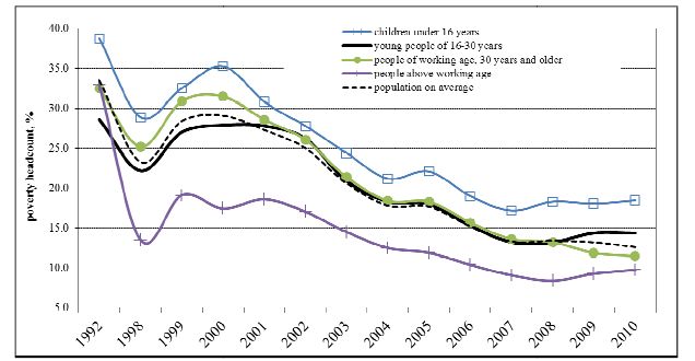
As far as the national poverty profile is concerned, children under 16 years are in the most vulnerable position (Figure 1). In 2010 the poverty headcount of this group was 1.5 times as high as the national poverty headcount. The gap between child and overall poverty measures has been growing throughout the 2000s: in 2000 the child poverty headcount was higher than the overall figure just by 20%. The poverty headcount of young people (16–30 years) is by 15% higher than the overall poverty measure. Risks of being poor for the working age adults over 30 years old are slightly lower than the average figure. Pensioners appear to be in the most privileged position: their poverty headcount is below the national average by 20%.

Poverty headcount in Russia by population groups, 1992–2010.
Source: Own calculations based on the FSSS data.
Such a distribution of poverty risks is typical for most Russian regions. The exceptions are the two major urban agglomerations of Moscow and St. Petersburg, where there are no deep problems on the labour market, and the ratio of average earnings and state pension is not in favour of the latter, so there it is the non-working young people (students and the unemployed) and pensioners who have a higher probability of falling into poverty. In the natural resources exporting regions, oriented primarily on male employment, lone-parent families are at the greatest risk of poverty. In virtually all territories, the most problematic group is families with 3+ children, but they are few in number, therefore do not predominate among the poor. The exceptions are the national republics in the South of Russia and the less developed Northern regions.
3. RUSMOD: The Russian microsimulation model
RUSMOD is the first full-scale model that permits simulation of most of the existing monetary policies implemented at federal and regional levels for the nationally representative sample of the population. The model is built on the EUROMOD platform (version F5.37). EUROMOD is continually being improved and updated (Immervoll & O’Donoghue 2009; Liets & Mantovani 2007; Sutherland 2001; Sutherland et al. 2008; Sutherland & Figari 2013). It has been previously successfully used as a platform to build microsimulation models for Serbia (Žarković-Rakić 2010) and South Africa (Wilkinson 2009). The construction and development of RUSMOD is documented in the EUROMOD Working Paper (Popova 2012).
Being a spin-off of EUROMOD, the Russian model has a number of advantages: (1) it captures the complexity of the Russian tax-benefit system, (2) it is flexible so that users are able to alter policy parameters and build in new policies, (3) it can be used for cross-national policy comparisons; (4) it can potentially become a platform for analyzing behavioral changes due to policy reforms. This marks a striking difference with respect to previous tax-benefit models for Russia, such as the one constructed within the UNU/WIDER project (Decoster 2003). Having been designed for the analysis of indirect taxes, that model simulated tax liabilities for the indirect Tax Code (social insurance contributions and personal income taxes were not simulated) and a limited number of social benefits. The user could only modify existing benefits, but could not add any new ones.
The aim of building RUSMOD was to simulate as many existing policies as possible. However, due to the data constraints not all the taxes and social benefits are simulated by the model. Firstly, some policies are beyond the scope of the model entirely or there is little or no data for that purpose, hence they are not included in the database. This refers to all indirect taxes and in-kind benefits (free or subsidized health care, childcare and other social services). Theoretically these elements can be accounted for within the model framework, as was demonstrated by a EUROMOD related project.5 However, they have been neglected, at least temporarily, to limit complexity and to keep model building a manageable task. Secondly, lump-sum allowances (e.g. the birth grant, the maternity capital, the funeral grant, etc.) are not simulated assuming that they do not affect current consumption of households. Thirdly, due to lack of the relevant data in the survey a number of allowances could not be simulated. Those include cash allowances for carers of the disabled persons and for families taking care of orphaned children. Finally, some allowances are available in the database and may be included in the disposable income, but the rules governing them may not be changed by the model. Those are benefits that depend on the long-term contribution history, including pensions and the social supplement to pension, the monetized privileges, the unemployment benefit and the temporary incapacity benefit.
Table 2 presents the order of simulation in the model. Social insurance contributions are simulated first, as they are defined as a percentage of withholding income tax base. All social benefits are not subject to taxation; hence they are simulated after the personal income tax. The maternity leave allowance and the child care allowance up to 1.5 years are included in any income test, hence have to be simulated first. Eligibility for means-tested benefits is derived from comparing disposable family/household income with the poverty line (Minimum Subsistence Level), which has to be simulated before means-tested benefits. Means-tested benefits are simulated in that particular order because the income test for the state social assistance takes account of the child allowance up to 16(18) years, while the means-test for the housing subsidy includes the state social assistance.
Order of simulation in RUSMOD, 2010.
| Policy name: | Short policy description: |
|---|---|
| Employer social insurance contributions (Страховые взносыработодателей) | Social insurance contributions (SIC) are paid by employers on behalf of employees to cover the costs of mandatory social insurance-based allowances, public pensions and health care. Contribution rates are set by the Federal laws. Social contributions apply to the withholding personal income tax base (i.e. gross earnings). Annual employment income below 415,000 Rubles is taxed at 26%, while income exceeding this amount is exempt. |
| Self-employed social insurance contributions (Страховые взносысамозанятых) | The size of contributions for self-employed people is determined as follows: Cost of annual insurance = Minimum Wage * SIC Rate *12. The monthly minimum wage equals 4,330 Rubles. The self-employed are obliged to pay only pension and health insurance contributions, participation in other social insurance programs is voluntary. |
| Personal Income Tax (Налог надоходы физических лиц) | Income taxation is individual. A unified tax rate of 13% applies to main income (work for pay, contractor’s agreements, housing lease). State pensions and allowances are normally not taxable. Capital gains from asset sales are taxable only if the seller owned the asset for less than 3 years. A higher tax rate of 35% applies to some sources of income, e.g. bank interests that exceed the upper limit computed using a refinancing rate. However, interest rates are usually below the threshold, making interests tax free. Dividends received by shareholders are subject to a 9% tax. The model differentiates between the withholding income tax and the final income tax. The former is the amount of an employee’s pay withheld by the employer and sent directly to the government as partial payment of income tax. For the latter the liability is based on the final tax report submitted at the end of each tax year (in April). There are two non-refundable tax allowances that are used to reduce the withholding income tax base (the standard tax allowance for each taxpayer and the standard tax allowance for taxpayer’s children). |
| Maternity leave allowance (Пособие по беременности иродам) | The allowance is paid to socially insured women for approximately 4 months (70 days preceding the child birth and 70 days after). The monthly size of allowance equals 100% of monthly earnings net of withholding income tax, with an upper limit of 34,583 Rubles per month (the upper limit of income base for SIC). |
| Child care allowance up to 1.5 years (Пособие по уходу за ребенком ввозрасте до 1.5 лет) | There are two types of this allowance. The contributory allowance is proportional to a mother’s net earnings for the last 6 months preceding the leave. The monthly size equals 40% of net earnings with an upper limit of 13,833 Rubles. There are two lower limits – 2,060.4 Rubles for the first child and 4,120.8 Rubles for the second and subsequent children. The non-contributory allowance is provided to all women who did not have any earnings in the last 6 months. The monthly size equals 1,798.5 Rubles for the first child and 3,597 Rubles for the second and subsequent children. |
| Compensation of charges for pre-school institutions (Компенсация части родительской платы за посещение ребенком учреждения дошкольного образования) | Cash compensation is provided to all families with children attending public or private pre-school institutions that provide a general education program. The size of compensation is proportional to actual fees paid by parents and amounts to 20% for the first child, 50% for the second child and 70% for the third and subsequent children. |
| Minimum Subsistence Level (Прожиточный минимум) | Eligibility for means-tested allowances is defined by comparing family/household income with the poverty line or Minimum Subsistence Level (MSL). The value of MSL is computed separately for three socio-demographic groups – children under 16 years, persons of working age (men 16–59 years, women 16–54 years) and persons of retirement age (men 60+ years, women 55+ years). The MSL is set quarterly in all Federation subjects according to the federal guidelines. |
| Child allowance up to 16(18) years for poor families (Пособие на детей до 16(18) лет из бедных семей) | A monthly means-tested allowance is paid to families with children below 16 years (or 18 years if they are in full-time education). The means test is applied to the sum of parents’ net earnings, scholarships, pensions and alimonies averaged over the last 3 months. According to the federal regulations the allowance must be provided in all regions, but the amounts are set by regional authorities. The model computes the allowance for 5 categories of families that are differentiated in most of the Federation subjects and are large enough to be detected in the sample, including: two-parent families, lone mothers, large families (families with 3+ children), families with disabled children and families with disabled parents. |
| State social assistance (Государственная социальная помощь) | The allowance is means-tested and targeted at poor households and households in hard life situation. This program is both regulated and funded by regional authorities and there is no minimum federal standard of service provision. The means test is typically applied to total household income from all sources, including net earnings, net investment income and income from lease, pensions, scholarships and other social allowances, averaged over the 3 preceding months. The most common eligibility rule is that the total household income should be below the (fraction) of the regional poverty line (MSL) due to circumstances that could not be prevented by the family. In other words, it means that all people of working age should provide a justification if they are currently not working and not seeking employment. The target group may be additionally narrowed down to certain categories of the population that are considered to be the most vulnerable in that particular region (e.g. lone mothers, pensioners living along, families with the disabled members). The size of allowance is usually computed as a (fraction) of the shortfall of the household income from the poverty line for that particular household. In some cases the size of allowance is set as a fixed amount per family member. It is not uncommon to define upper and lower limits. |
| Housing subsidy (Жилищная субсидия) | This is a partially means-tested benefit designed to assist low-income households with meeting the costs of rent and utilities. Income test is applied to the total household income from all sources (as for the state social assistance) averaged over the last 6 months. The computation formula is quite complicated and includes a number of conditions at household and regional levels. The size of allowance is equal to: (social standard of living space*N of persons in the household * social standard of the cost of rent and utilities per 1 square metre) – (household income * maximum share of the cost of rent and utilities in total household income). For non-poor households, i.e. those whose income is equal or over the regional MSL, and for households eligible for discounts on rent and utilities, the formula is additionally multiplied by adjustment coefficients to reduce the subsidy size. The latter cannot exceed the actual cost of rent and utilities. The subsidy is only available if the household has no debts for rent and utilities. Social standards of the cost of rent and utilities are set by regional authorities. The maximum share of the cost of rent and utilities in household income may not exceed 22%. |
-
Notes: Exchange rate = 40.3 Rubles per 1 Euro (2010); PPPs (household consumption) = 16.2 Rubles per 1 Euro (2008); Net average monthly earnings = 20,437 Rubles (2010). Detailed description of the Russian tax-benefit system, including policies that are not simulated in RUSMOD is available in Popova (2012).
-
Source: Own analysis of the federal and regional legislative acts.
It should be borne in mind that the level of precision in replicating the exact policy rules depends to a large extent on the level of control over the program by the federal authorities. The precise simulation of social insurance contributions and the personal income tax is quite straightforward due to the transparency and high level of centralization of the Russian tax system. Allowances paid from the Social Insurance Fund are simulated relatively precisely. As far as means-tested programs are concerned, the rules for housing subsidies (mainly subject to federal legislation) are simulated more precisely compared to child allowances (subject to regional legislation but with minimum standards set in the federal law). The state social assistance which is provided completely at the discretion of regions has to be simulated with many simplifications and assumptions.
In order to be used within the EUROMOD framework the input dataset has to meet certain requirements (Figari et al. 2007). A number of national household surveys have been considered for this purpose and the only one that fulfilled all the essential conditions was the Russian Longitudinal Monitoring Survey (RLMS-HSE)6 most recently conducted in 2010 (Table 3). Until recently, the RLMS was the only freely available dataset and the main source of all empirical research on poverty in Russia. It is a typical multi-topic survey with an extended set of information on economic well-being and health status. It collects individual level information on demographic characteristics, within-family relationships, labour market status, primary income by source, social benefits (including those that cannot be simulated), and also expenditure and other relevant characteristics that may affect tax liabilities or benefit entitlements. Since December 1994 data are collected once a year by the Institute of Sociology of the Russian Academy of Sciences. Initially the survey was managed by the University of North Carolina and satisfies international standards in terms of sampling and quality of data collection. The sample includes both cross-sectional and panel components and is large enough to support the analysis of small groups at the national level. The current version of RUSMOD uses the 2010 cross-sectional sample which consists of 6,323 households and 16,867 individuals. In geographical terms it covers 32 (out of 83) Federation subjects and is not representative at the regional level, which is the main limitation of the survey.
RUSMOD input database description, 2010.
| Original name | Russian Longitudinal Monitoring Survey (RLMS-HSE) |
|---|---|
| Provider | National Research University – Higher School of Economics |
| Year of collection | 2010 |
| Period of collection | October-December 2010 |
| Income reference period | Typically income and expenditure for the month preceding the survey, for some types of expenditure – 3 months preceding the survey |
| Sampling | A three-stage stratified clustered probability sample of dwellings |
| Unit of assessment | Household (people living together and sharing income and expenses) |
| Coverage | Permanent residents, people living in institutions are excluded |
| Sample size | 21,343 individuals; 7,923 households (total sample including the panel element) |
| Response rate for household grid | 80% (60% in Moscow and St-Petersburg) |
| Final sample used in the model | 16,867 individuals; 6,323 households |
| Weighting | The weights must be used in order to adjust the sample for design factors (sampling probabilities and non-response) and deviations from the census characteristics. In addition, the weights provided with the original data were scaled up to the overall population |
The official poverty figures in Russia are based on the Household Budget Survey (HBS). It is conducted on a sample of 50,000 households, carried out continuously on a quarterly basis in 82 Federation subjects (excluding the Chechen republic). There is a large non-response and re-weighting of data. The sample is clustered, small at the regional level and has some serious coverage problems for a number of Russian regions. When it comes to building a microsimulation model, the main disadvantage of HBS is the limited questionnaire. The main purpose of the survey is to collect information about the average consumption pattern of the population in order to provide weights for the consumer price indices and calibrate the household account from the system of National Accounts. HBS was not designed for income distribution analysis. It collects detailed information on household purchases, consumption and capital transactions, plus a limited set of information about household composition. Data on individual sources of income, such as earnings, pensions, social benefits, are not collected since 1997, because they are considered a priori unreliable.
In 2003 with the support of the World Bank the national statistics agency has carried out the Sample Survey of Household Welfare and Participation in Social Programs (NOBUS). NOBUS combined the advantages of RLMS-HSE (integrated questionnaire) with those of HBS (regionally representative sample of 44,000 households). This is best practice survey but it is outdated.
Another potential source was the Gender and Generation Survey carried out in 2004, 2007 and 2011 by the Independent Institute for Social Policy. The survey covers 11,000 respondents and is aimed at collecting the detailed information about the history of demographic and employment behavior of individuals, while the data on income and social programs are much less detailed than in RLMS-HSE. The GGS sample is compatible with the RLMS-HSE sample, thus in future development of RUSMOD the two surveys could be merged in order to simulate the behavioral responses to policy incentives.
In the future regional surveys can be used to address the problem of lack of regionally representative data sources. The most rigorous attempts covering sufficiently large number of respondents based on scientific sampling and integrated questionnaires were made in 2005 in Leningrad region (2,500 households) and in 2006 in Tomsk region (3,000 households), both financed by grants of the UK Department for International Development. In 2012 the Government of Moscow has launched the program of comprehensive household surveys (covering 3,000 households) with an emphasis on accurate measurement of household well-being and participation in social programs.
4. Data adjustment and model validation
Validating simulation output against official statistics (National accounts and administrative data) is a necessary step in assessing the robustness of the microsimulation model and its applicability for policy analysis. To ensure comparability with the external sources several adjustments were made to the original RLMS-HSE data, apart from the imputation of user-missing data. They are discussed in this section.
First of all, it should be noted that due to some country-specific labour market mechanisms the correct measurement of earnings in surveys and, hence, the correct simulation of taxes and SIC in Russia is quite problematic. For the majority of Russian firms both in public and private sector, over a third of total earnings is variable and not fixed in labour contracts (Gimpelson & Kapeliushnikov 2011). This part comprises premiums and bonuses that can fluctuate contingent upon general economic conditions and firm performance. In case of economic slowdown, the variable part of earnings shrinks, while in the upturn the employees are likely to enjoy an additional premium. In addition, Russian firms might use informal (undeclared) payments in order to cut costs related to SIC. This part of earnings is not bound by any formal constraints and is even more sensitive to changes in economic conditions. According to the national statistics agency, throughout the 2000s the share of earnings hidden from statistical observation, i.e. unreported earnings, made up about 30-40% of the official (declared) earnings7, ranging from less than 15% in the bottom income decile to over 50% in the top income decile (UNDP 2011). These unreported earnings are imputed and included as an element of total population income in macro-statistics. Noteworthy, this is something else than the hidden or the illegal economies. The latter comprise the activities related to tax fraud or tax evasion or illegal activities. The non-observed economy also comprises activities that have nothing to do with criminality or tax evasion, but that still remain unobserved because the traditional survey tools are not perfect (non-response, under-reporting, short income reference period) and business registers are not always complete and up-to-date.
RLMS-HSE attempts to capture the informal sector jobs, which appear to be quite widespread, especially for the additional jobs. Among employees the share of those who reported that they did not have a formal contract amounted to 6.6% at the main job and 32% at the second job. For self-employed people the share of those who reported that they were working without registration was 17.2%. Over 80% of those who had occasional jobs worked without a formal contract. In the computations of taxes and contributory benefits the earnings of informal sector workers were set to zero.8 The total amounts of both SIC and income tax were predicted quite precisely (Table 4). Yet a large share of earnings of both informal and formal sector workers is likely to remain unaccounted for by the survey due to the atypical composition of earnings in Russia (large variable part) or due to the deliberate non-response or under-reporting by the respondents. The poverty rate in RLMS-HSE was overestimated compared to official statistics (23% against 12.6%), and so was the coverage of means-tested programs. That is why an additional calibration of disposable income was needed.9
Model validation: simulation of taxes and benefits in the original and calibrated scenarios, 2010.
| Taxes and social benefits: | Original data | Simulation scenarios: | External source | |
|---|---|---|---|---|
| original | calibrated | FSSS | ||
| Social insurance contributions | ||||
| recepients, % of population | n/a | 42.8 | 42.8 | n/a |
| mean size, Rubles | n/a | 3,999 | 3,999 | n/a |
| expenditure, mln Rubles | n/a | 2 820,000 | 2 820,000 | 2 562,974 |
| Personal Income Tax | ||||
| recepients, % of population | n/a | 44.7 | 44.7 | n/a |
| mean size, Rubles | n/a | 2,413 | 2,413 | n/a |
| expenditure, mln Rubles | n/a | 1 776,000 | 1 776,000 | 1 789,600 |
| Maternity leave allowance | ||||
| recepients, % of population | n/a | 0.1 | 0.1 | 0.7 |
| mean size, Rubles | n/a | 13,676 | 13,676 | n/a |
| expenditure, mln Rubles | n/a | 33,000 | 33,000 | 67,317 |
| Child care allowance up to 1.5 | ||||
| years | ||||
| recepients, % of population | 1.3 | 1.6 | 1.6 | 2.6 |
| mean size, Rubles | 4,086 | 3,599 | 3,599 | n/a |
| expenditure, mln Rubles | 90,720 | 94,800 | 94,800 | 121,797 |
| Compensation of child care | ||||
| charges | ||||
| recepients, % of population | 2.8* | 2.6 | 2.6 | 3.0 |
| mean size, Rubles | 1,055 | 388 | 388 | n/a |
| expenditure, mln Rubles | 49,440 | 16,680 | 16,680 | n/a |
| Child allowance up to 16(18) | ||||
| years | ||||
| recepients, % of population | 4.4 | 7.0 | 4.6 | 4.7 |
| mean size, Rubles | 962 | 583 | 622 | n/a |
| expenditure, mln Rubles | 70,440 | 66,960 | 46,680 | 43,081 |
| State social assistance | ||||
| recepients, % of households | 1.0 | 3.7 | 1.0 | 1.0 |
| mean size, Rubles | 2,233 | 1,713 | 1,437 | 796 |
| expenditure, mln Rubles | 15,000 | 41,520 | 9,264 | n/a |
| Housing subsidy | ||||
| recepients, % of households | 8.5 | 24.4 | 7.1 | 7.3 |
| mean size, Rubles | 1,018 | 1,040 | 822 | 896 |
| expenditure, mln Rubles | 56,280 | 165,600 | 38,280 | 55,719 |
-
Notes:
-
*
children attending pre-school institutions and actual fees.
Official data on poverty in Russia faces similar inconsistencies. As mentioned in Section 3, the source of original data for assessing income distribution is HBS. Since 1997 HBS collects data on consumption only. The preference to use consumption as welfare indicator is dictated by country-specific considerations. As in other transition economies, in Russia consumption data is collected more reliably than income data (Deaton 1997). The latter tends to suffer from incomplete measurement, under-reporting, and seasonality. Some regular (non-seasonal) sources of income, such as earnings of formal sector workers and social transfers, are quite accurately measured by surveys. More volatile sources, such as the variable and/or informal part of earnings, income from subsistence farming or some types of self-employment, are poorly captured by surveys (Ovcharova & Tesliuk 2006). This is true for HBS and it also true for other household surveys. Noteworthy, another study using RLMS-HSE for 1994-2006 have concluded that estimates of household welfare based on expenditure are more reliable: they are consistently higher and less volatile than those based on income (Gorodnichenko et al. 2010).
By various estimates the HBS sample does not cover from 5 to 10% of the Russian population, including the poorest and especially the richest households. To deal with this fact, the welfare aggregate derived from HBS is statistically manipulated to match macro-level estimates of income using a two-parameter lognormal model. One of the parameters of this model – a root mean square deviation of logarithms – is derived from HBS, another parameter – mean per capita income – is taken from National accounts. Due to the adjustment for unreported earnings the mean income in National accounts is considerably higher than the expenditure aggregate in HBS. As a result, poverty and inequality estimates in the macro-statistics are lower than those derived from the original HBS data, although the mean income is higher. The appropriateness of using the lognormality assumption for modeling the distribution of income in the present situation of Russia is a most debatable issue. At the same time, comparing RUSMOD output with the official statistics is the only way to check the validity of the model in terms of income distribution estimates.
Following the logic of the national statistics agency, i.e. assuming that the data on expenditure are more reliable, in the calibrated income scenario a special function was introduced to impute the unreported income. To arrive at this estimate all the components of income reported in the survey, including employment income of formal sector workers, pensions, social benefits, private transfers, investment income and lump-sum income were summed up. This sum was then deducted from the household consumption aggregate.10 If the result of this function was higher than zero it was treated as the unreported income. For 17% of Russian households the reported expenditure appeared to exceed the reported income. The share of those with under-reported income ranged from 15% in the bottom income decile to 25% in the top decile. On average the imputed amount was equal to 20% of the total household income (from 19% in the bottom income decile to 30% in the top decile). Although this method is more straightforward, the scale of income adjustment is similar to that made by the national statistics agency. The inclusion of unreported income in the simulated disposable income solved the problem of the inflated poverty rate. The poverty headcount which was equal to 23.4% before income imputation dropped to 12.9% after income imputation, which is similar to the official figure (12.6%).
The unreported income was then included in the means test for two allowances11 – the state social assistance and the housing subsidy – as a proxy for household assets. Given that the information on assets reported in the survey is limited compared to that available to local Social protection offices and given the positive correlation between household assets and unreported income, the inclusion of the latter enables us to simulate the means test more precisely. However, even after the income adjustment the share of households eligible for means-tested allowances remained inflated, which resulted in underestimation of the poverty headcount after the simulations (11.8% versus 12.6% according to macro-statistics). The numbers of recipients were higher than those reported in administrative statistics by 30% for the child allowance and by around 50% for the state social assistance and the housing subsidy. Unfortunately, the administrative statistics does not collect any information about non-take up rates12 of means-tested benefits and this topic has not been researched so far. Thus, the only option was to rely on theoretical considerations and evidence from other countries. For a few OECD countries for which estimates are available, they range between 20 and 60% in case of social assistance and housing programs and 20 to 40% in case of insurance-based unemployment benefits (Hernanz et al. 2004), which is similar to the situation observed in Russia.
Theoretically the non-take up of means-tested programs may reflect both demand and supply side problems. The former arise when for some reasons eligible households choose not to apply for benefits. The ‘voluntary’ non-take up may happen due to lack of knowledge about the available social programs and high costs associated with the claim, e.g. complicated administrative procedures or social stigma (Moffitt 1983). It is more likely to happen when the benefit amounts are low compared to the costs of applying, which is true for all means-tested allowances in Russia. A typical example of a supply side problem is when due to lack of funds the welfare administration is compelled to ration the benefits. The Russian program of state social assistance makes a good illustration. Since it is fully regulated and funded by regions, the number of those who receive the cash benefit is limited by financial constraints of the Regional Budgets. In many regions applications are accepted up to a budget limit and local authorities have discretion to refuse applications.13
Another possible source of error is that the simulation procedures used to identify the eligible population in the dataset are far from perfect. The input dataset is a general-purpose household survey which was not designed to collect information about eligible non-claimants (e.g. the amount of benefits not claimed, the duration of eligibility for programs, existence of stigma associated with the claim, etc.). Thus, the eligibility can only be determined through imputation procedures based on household characteristics and income and those are not always as detailed as it is necessary, while administrative rules governing eligibility are quite complex. For example, the means test for the state social assistance and housing subsidies has to be applied to household income averaged over the last 3 or 6 months, respectively, yet the survey collects information only about income for the month preceding the survey, and the simulations assume that this amount of income is received by the household throughout the year. This is a quite strong assumption for Russia, where the large part of earnings is variable. There is another imprecision in simulation of housing subsidies. In order to be eligible each household member has to provide a proof of registration at this particular address. Unfortunately, information about the registration status of household members was not collected, so the simulations assume that that all household members residing in the dwelling are eligible which might not be true in reality.
Since it is impossible to disentangle the relative contribution of different factors in explaining the over-prediction of the number of beneficiaries of means-tested programs, a random non-take up correction was employed. The take up probabilities were estimated as the ratio between the caseload recipients reported by administrative statistics and those simulated to be entitled by RUSMOD (68% for child allowances, 51% for the state social assistance and 46% for housing subsidies, respectively). Those probabilities were applied at the household level (so that people entitled to the same benefits within a household exhibit the same take-up behaviour), for each means-tested benefit separately.14 This method is very rough and does not satisfactorily reflect the real take up issues at play (large discretionary power of local Social protection offices, detailed assets test). However, as mentioned above, the input dataset is a general-purpose survey which is not applicable for econometric modeling of take up. The refinement of this is one of the planned future developments of the model.
Table 4 demonstrates that the calibrated simulation scenario (assuming income under-reporting and a random non-take up of means-tested allowances) produces a better match between the components of the model and administrative statistics, as well as between the model and the actual survey data, compared to the original simulation scenario (assuming no income adjustment and 100% take up of means-tested benefits).
Without adjustment for unreported income poverty estimates simulated by RUSMOD were too high relative to official poverty statistics, and without the additional correction for non-take up they were too low. Table 5 demonstrates that the calibration of income together with the nontake up adjustment produces a much better match. The overall poverty headcount is 12.4% compared to 12.6% according to macroeconomic statistics. The child poverty headcount is 19.3% compared to 18.5%. The poverty rate of young people (16–30 years) is 14.7% against 14.4%. Comparisons for older people are less good, but are still close: the poverty headcount for adults below retirement age (30–54/59 years) is 13.5% against 11.5%; for pensioners – 4.2% versus 9.8%.
Model validation: simulation of income inequality and poverty in the original and calibrated scenarios, 2010.
| Simulation scenarios: | External source | |||||
|---|---|---|---|---|---|---|
| Original | Calibrated | HBS 2010 | FSSS 2010 | |||
| RLMS-HSE | RUSMOD | RLMS-HSE | RUSMOD | |||
| Mean disposable income, | 12,625 | 12,641 | 15,720 | 15,723 | 12,898 | 22,140 |
| Rubles | ||||||
| Gini coefficient | 0.421 | 0.416 | 0.422 | 0.421 | 0.421 | |
| Decile ratio (9th to 1th), times | 6.0 | 5.6 | 5.1 | 5.0 | 7.4 | |
| Income distribution: | ||||||
| 1st quintile | 5.3 | 5.6 | 6.2 | 6.3 | 6.9 | 5.2 |
| 2nd quintile | 10.7 | 10.8 | 10.7 | 10.7 | 11.0 | 9.8 |
| 3rd quintile | 15.1 | 15.1 | 14.3 | 14.3 | 15.5 | 14.8 |
| 4th quintile | 21.0 | 20.9 | 19.7 | 19.7 | 23.8 | 22.5 |
| 5th quintile | 47.8 | 47.6 | 49.1 | 49.1 | 42.8 | 47.7 |
| 10th decile | 33.4 | 33.2 | 35.1 | 35.0 | 26.0 | 30.9 |
| Poverty headcount, % of the population: | 23.8 | 22.2 | 12.9 | 12.4 | 12.6 | |
| Children under 16 years | 37.5 | 35.0 | 20.3 | 19.3 | 18.5 | |
| Young people aged 16–30 years | 27.7 | 26.5 | 15.0 | 14.7 | 14.4 | |
| People over 30 years and below state pension age | 26.3 | 24.4 | 14.1 | 13.5 | 11.5 | |
| People over state pension age | 7.7 | 6.9 | 4.3 | 4.2 | 9.8 | |
| Poverty gap, % of total income of the population | 6.0 | 5.2 | 2.1 | 2.0 | 1.2 | |
-
Notes: All indicators are calculated using per capita disposable income because the Russian official statistics does not apply any equivalence scale; the poor are those whose per capita disposable income is below the Minimum Subsistence Level.
In a similar way to poverty estimates, calibration improves the match of other income distribution characteristics in the model both with macro-statistics and the original survey data. In the calibrated simulation scenario the share of the top income quintile appears to be higher than the official number (49.1% versus 47.7%). The estimates of the income share of the top decile diverge even more seriously (35% in the model versus 30.9% in National Accounts). At the same time, the bottom quintile has a higher income share in RUSMOD (6.3% versus 5.2%). The decile ratio in RUSMOD is lower (5 times against 7.4 times in macro-statistics), while the values of Gini coefficient are identical (0.421). Noteworthy, in case of Russia it is impossible to achieve completely identical results, because of the macro-statistics’ recourse to additional statistical manipulations, such as the lognormality assumption, to account for the sample bias.
Summarizing, after the calibration RUSMOD produces reliable estimates of taxes, benefits and income distribution characteristics given the data constraints. However, the assumptions made in the process of calibration should be borne in mind when planning appropriate uses of the model and in interpreting results. Limitations applicable to all arithmetic microsimulation models apply to the Russian model as well. In particular, the simulation of long-term effects of policy reforms, apart from the incentive potential of the tax-benefit system, are beyond the scope of the model.
5. Model application: the distributive impact of alternative reforms of child allowances
There was a significant progress in poverty reduction in Russia since 2000 due to rapid economic growth. At the same time, poverty has been changing its face: it is now increasingly concentrated in rural areas, among the low educated and households with high dependency load and weak ties with the labour market (e.g. families with many children). Given these structural characteristics economic growth alone cannot eliminate extreme forms of poverty, but needs to be supplemented by targeted and efficient safety nets. This section starts by introducing all existing anti-poverty programs and discussing their redistributive impact. Noteworthy, there is no such thing in Russia as a single anti-poverty benefit, instead there are three programs where poverty and other eligibility criteria are mixed.
Child allowances are provided to children in families with per capita income below the regional poverty line. This is a classical example of anti-poverty program. It was introduced in 1994 and was initially granted to all children up to 16 years (or 18 years if they are in full-time education).
In 1998 the first income test was introduced which limited the number of recipients by families whose income was below 200% of a regional poverty line (100% of a regional poverty line since 2000). Such a measure was aimed at providing better redistribution of scarce financial resources in the interests of the poorest families with children. Nevertheless, the targeting accuracy of the program is low. As a result, the program fails to provide adequate support to participating families (the average size of the benefit per household amounts to about 10% of the MSL), while spreading its budget to a large number of children, 65% of whom are not poor. Another problem is high regional disparities in the benefit amounts. In 2010 the gap in basic monthly payments between the most generous and the least generous region amounted to 14 times.
Housing subsidies on the other hand, have a more complex objective. They were originally introduced in 1994 to mitigate social consequences of moving to 100% cost recovery across the country, so as to ensure that the utility sector smoothly received payments for the services it provided to the population, despite higher tariffs for utilities. This objective is not directly related to poverty reduction. At the same time, the program was designed to protect people from spending a high share of their income on rent and utilities, using an imperfect concept of equity. A household with housing costs in excess of the regional threshold (no less than 22% of household income) would qualify for a subsidy that would bring the share of housing costs down to the threshold. Eligibility and benefit formulae allow non-poor to qualify as beneficiaries.
In 1999, federal legislation was expanded to include the program of state social assistance, whereby introducing the concept of targeting resources to the poor. The program design and the decisions as to whether to target any benefits to the poor alone have been left with regional authorities. Currently, significant design problems are found in the legislative acts stipulating the rules for the regional and municipal programs. Most often the rules mix the notion of targeting with categorical provision of assistance, defining certain groups (such as lonely pensioners, families with 3+ children, student families etc.) who are eligible for the benefits. In addition, targeted assistance is often confused with one-time emergency assistance provided in force majeure situations (e.g. loss of the breadwinner, severe illness, natural disaster). The scale and type of help depends greatly on the priorities and financial constraints of regional authorities, thus interregional variation in spending on this program is the highest among the means-tested programs.
RUSMOD may be applied to check how effective these programs are in terms of reducing poverty and inequality. For that purpose the benefits are consecutively ‘removed’ from the national tax-benefit system. The rest of policies remain in place and interact with each other. By comparing poverty outcomes with and without selected cash transfers the first-order poverty effects of the existing arrangements can be evaluated. Poverty is assessed using the national poverty concept, whereby the poverty line equals the MSL which is set quarterly by each region according to the national guidelines. By definition the poverty line is maintained fixed across all the scenarios. Two poverty indices are used – the traditional poverty headcount and the poverty gap, i.e. the average shortfall in income of the poor from the poverty line (Ravallion 1992). They are computed for the entire population, for children under 18 years and for the most vulnerable group – households with 3+ children.
The three means-tested allowances simulated by RUSMOD in total account for 0.2% of GDP. The most expensive one is the child allowance which accounts for 50% of the overall spending. About 40% of the budget is spent on housing subsidies. The cost of the state social assistance is estimated as 10% of the overall spending on the three means-tested programs (Table 6). Altogether the three programs reduce the national poverty headcount and poverty gap measures by 6 and 5%, respectively. The child poverty headcount and poverty gap measures are reduced by 7 and 6%, respectively. Having limited effect on the poverty rate of large families, the means-tested programs still reduce their poverty gap by 10%. By far the largest contribution to poverty reduction is made by child allowances. The total reduction in Gini coefficient due to all three programs is below 1%. This sharply contrasts with the situation in European countries, where means-tested transfers reduce inequality by 10% on average (Immervoll et al. 2006).
Policy impact of means-tested benefits, baseline policies, 2010.
| Child allowance up to 16(18) years | State social assistance | Housing subsidy | All means-tested programs | |
|---|---|---|---|---|
| Policy characteristics: | ||||
| Beneficiaries, % of households | 11.5% | 1.0% | 7.1% | 6.8% |
| Mean size per household, % of MSL | 10.9% | 24.4% | 13.9% | 14.2% |
| Expenditure, % of GDP | 0.09% | 0.02% | 0.07% | 0.17% |
| Vertical efficiency, % of the poor among beneficiaries | 35.3% | 93.1% | 39.8% | 43.6% |
| Policy impact (% change in the indicator due to the program): | ||||
| Gini coefficient | −0.2% | 0.0% | −0.2% | −0.7% |
| National poverty headcount | −2.4% | −0.8% | −1.6% | −5.6% |
| National poverty gap | −1.8% | −1.1% | −1.8% | −4.6% |
| Poverty headcount, children under 18 years | −3.7% | −1.6% | −1.6% | −6.9% |
| Poverty gap, children under 18 years | −3.1% | −1.0% | −2.4% | −6.1% |
| Poverty headcount, couples with 3+ children | 0.0% | 0.0% | −2.2% | −2.0% |
| Poverty gap, couples with 3+ children | −7.4% | −2.7% | 0.0% | −10.0% |
-
Source: Own calculations based on RUSMOD.
In 2010, more than 15% of all the money spent on means-tested programs accrued to beneficiaries from the two upper deciles (Figure 2). Only 35% of recipients of child allowances and 40% of recipients of housing subsidies were poor. In terms of targeting efficiency, the least problematic program is the state social assistance (93%), but it has a low share in total spending. In total over 50% of resources earmarked for three programs are spent on non-poor beneficiaries. This is an extremely weak targeting performance when compared internationally. In OECD countries and in many middle income countries as well, cash transfer programs aimed to reduce poverty have a smaller share of non-poor beneficiaries, below 35%, or in case of the best programs, below 20% of their caseloads (Weigand & Grosh 2008).
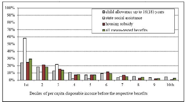
Distribution of the total spending on means-tested benefits by income deciles, baseline policies.
Source: Own calculations based on RUSMOD.
These modest results occur because by design the two most generous programs – child allowances and housing subsidies – include non-poor beneficiaries in their target groups, while the program of state social assistance which is the least problematic in terms of targeting, does not receive enough funding. The way the programs are currently designed make them ineffective means to achieve their goals, such as supporting families with children, helping poor households warm their houses during the cold season and providing a safety net for poor households.
Redirecting the resources spent on the non-poor to those in need by means of improving the program design could have a sizable impact on poverty reduction. RUSMOD can be used to simulate hypothetical reforms of means-tested benefits and to assess their impact on income distribution and poverty outcomes. Although all the programs could benefit from restructuring, raising the income of families of young disadvantaged children is likely to be a key part of portfolio of policy solutions to reduce poverty in Russia. In most regions it is households with children who constitute the majority of the poor. Several studies show that families with children have the higher probability of being poor and the higher poverty gap compared to other groups of households (Ovcharova & Popova 2005; Ovcharova et al. 2007; UNICEF 2011). The most vulnerable groups are families with high dependency ratio, i.e. families with 3+ children. They are more likely to experience repeated poverty spells. Noteworthy, in rich and other middle income countries child poverty is also a central issue for policymakers (UNICEF 2005, 2007; Richardson et al. 2008). All industrialized countries introduced comprehensive cash allowances for children to target child poverty (Bradshaw 2010; OECD 2009; Figari et al. 2011).
Hence, this paper focuses on improving the design of child allowances. We start by concentrating the same budget on the poor children, thus increasing the benefit amounts (Table 7). Scenario 1 concentrates on increasing the targeting accuracy, keeping the regional differences in the program design intact, and uses the released funds to finance the proportional raise in the benefit amounts. In the baseline implementation a child is eligible for the cash benefit if her/his parents’ income from employment, pensions and other social benefits is below the poverty line (option 1). Secondly, we limit the number of beneficiaries by those children whose total household income from all sources is below the poverty line (option 2). Thirdly, we reduce the number of eligible children to those whose total household income is below 75% of the poverty line (option 3). Scenario 2 addresses the issue of inter-regional disparities in the benefit amounts and implements the reform whereby the amounts are set at the federal level and do not vary across regions.15 Scenario 3 does the same simulations at the national level with the amounts adjusted by a coefficient accounting for differences in the cost of living across regions.16 All the simulated reforms are budget-neutral, i.e. do not change the overall budget of the program. The non-take up correction is switched off in all the scenarios.
Simulated reforms of child allowances.
| Size of allowance | |||
|---|---|---|---|
| Eligibility: | Scenario 1 – regionally set amounts | Scenario 2 – federally set nominal amounts | Scenario 3 – federally set amounts adjusted for regional PPPs |
| Option 1 – parents income below the poverty line | Baseline/Reform 1.1 | Reform 2.1 | Reform 3.1 |
| Option 2 – household income below the poverty line | Reform 1.2 | Reform 2.2 | Reform 3.2 |
| Option 3 – household income below 75% of the poverty line | Reform 1.3 | Reform 2.3 | Reform 3.3 |
In the second round of simulations, we implement the same nine reforms of child allowances with an increased budget. The budget increase is financed by another reform which improves the targeting of housing subsidies. In other words, we change the design of housing subsidies by excluding non-poor households from the number of eligible groups and by redirecting the released funds to the program of child allowances. As a result of this reform the total number of recipients of housing subsidies is reduced by 3.86 times and the total spending on housing subsidies is reduced by 2.7 times. At the same time the budget of child allowances is increased by 1.81 times (from 0.12 to 0.22% of the GDP) for the same number of beneficiaries. We repeat all the reforms described in Table 7 with the increased budget and compare their impact with the baseline implementation. All reforms are still budget-neutral in respect to the whole system of means-tested allowances.
Irrespectively of the reform, switching to a stricter income test implies a reduction in the number of program beneficiaries: from 18% of households in the baseline simulation (parents’ income below the poverty line), to 5.5% if option 2 (total household income below the poverty line) is implemented, and to 2.7% if option 3 (total household income below 75% of the poverty line) is implemented (Table 8). This allows us to reallocate the budget so that the average benefit amounts are increased: from 10% of the MSL under baseline/option 1, to 32% under option 2, to 67% under option 3.
Policy impact of the simulated reforms of child allowances under the current budget, 2010.
| Name of scenario: | baseline | reform 1.2 | reform 1.3 | reform 2.1 | reform 2.2 | reform 2.3 | reform 3.1 | reform 3.2 | reform 3.3 |
|---|---|---|---|---|---|---|---|---|---|
| Policy characteristics: | |||||||||
| Beneficiaries, % of households | 17.6%* | 5.5% | 2.7% | 18.1% | 5.4% | 2.7% | 18.1% | 5.4% | 2.7% |
| Mean size, % of MSL | 10.2% | 32.8% | 66.7% | 9.9% | 32.9% | 66.4% | 9.9% | 32.8% | 66.4% |
| Expenditure, % of GDP | 0.12%* | 0.12% | 0.12% | 0.12% | 0.12% | 0.12% | 0.12% | 0.12% | 0.12% |
| Vertical efficiency, % of the poor among beneficiaries | 34.0% | 94.8% | 99.8% | 38.5% | 99.1% | 99.8% | 42.4% | 98.6% | 100.0% |
| Policy impact (% change in the indicator due to the program): | |||||||||
| Gini coefficient | −0.3% | −0.3% | −0.3% | −0.3% | −0.3% | −0.1% | −0.3% | −0.3% | |
| National poverty headcount | −5.1% | 0.8% | 0.8% | −7.9% | 0.8% | 0.8% | −6.3% | −0.4% | |
| National poverty gap | −3.3% | −12.2% | −12.2% | −3.0% | −14.5% | −3.0% | −5.4% | −12.3% | |
| Poverty headcount, children under 18 years | −8.9% | 0.6% | 0.6% | −11.8% | −0.8% | 0.3% | −11.2% | −4.0% | |
| Poverty gap, children under 18 years | −5.0% | −19.7% | −19.7% | −3.7% | −24.6% | −5.4% | −9.7% | −20.3% | |
| Poverty headcount, couples with 3+ children | −8.7% | −6.4% | −2.5% | −21.2% | −15.1% | −5.3% | −33.5% | −31.2% | |
| Poverty gap, couples with 3+ children | −7.2% | −21.9% | −2.3% | −9.1% | −41.6% | −10.2% | −20.0% | −39.6% | |
-
Notes:
-
*
The number of beneficiaries and total expenditure on the program is higher than those in Table 6 because the take up correction is switched off.
Source: Own calculations based on RUSMOD.
Now we turn to the comparisons of outcome indicators by reform. Table 8 shows that even under the current budget of child allowances, a sizable reduction in all poverty indicators could be achieved if the benefit amounts were set at the federal level (scenarios 2 and 3). The second important conclusion is that holding the current budget constant, with stricter income test (options 2 and 3) poverty indicators could be lower than they are at present. The largest reduction in the overall poverty headcount (by 8%) and the child poverty headcount (by 12%) is observed if the amounts are flat and the allowance is paid only to those whose household income is below the poverty line (reform 2.2). However, poverty gap indices are less sensitive to this reform: there is just a 3% reduction in the overall poverty gap and a 4% reduction in the child poverty gap. The stricter income test (reform 2.3) brings about a greater reduction in the poverty gap for the whole population (14.5%) and children (by almost 25%), but it comes at the price of almost no change in the national and child poverty headcounts.
Additional adjustment of the benefit amounts to the cost of living in the region (reform 3.2) is slightly less beneficial in terms of the national poverty headcount (a 6% reduction), while the national poverty gap is reduced by 5%, which is an improvement over reform 2.2. In terms of the child poverty headcount reform 3.2 is almost as effective as reform 2.2 (an 11% reduction), and it is twice as effective in terms of the child poverty gap (a 10% reduction). Finally, none of the reforms is as beneficial for households with 3+ children as reform 3.2: the poverty headcount of this group is reduced by 33.5% and their poverty gap – by 20%. Although stricter income test (reform 3.3) brings about an even higher reduction in the poverty gap of families with 3+ children (40%), there is a substantial loss as far as all other poverty indicators are concerned, compared to reform 3.2.
Under the increased budget the average benefit amounts rise from 18% of the MSL under option 1, to 60% under option 2, and to 120% under option 3 (Table 9). Changes in the program design are the same as in the first set of reforms (with the constant budget), so the previous conclusions are reinforced. The introduction of the national benefit amounts adjusted for regional PPPs and narrowing the eligibility to those with household income below poverty line (reform 3.2) appears to be most beneficial in terms of the majority of our poverty measures. Under this reform the national poverty headcount and poverty gap measures fall by 15 and 6.5%, respectively; the child poverty headcount and child poverty gap measures fall by 25 and 12%; and families with 3+ children enjoy a 50% reduction in their poverty headcount and a 39% reduction in their poverty gap.
Policy impact of the simulated reforms of child allowances under the increased budget, 2010.
| Name of scenario: | reform 1.1 | reform 1.2 | reform 1.3 | reform 2.1 | reform 2.2 | reform 2.3 | reform 3.1 | reform 3.2 | reform 3.3 |
|---|---|---|---|---|---|---|---|---|---|
| Policy characteristics: | |||||||||
| Beneficiaries, % of households | 17.6% | 5.5% | 2.8% | 18.1% | 5.4% | 2.7% | 18.1% | 5.4% | 2.7% |
| Mean size, % of MSL | 18.5% | 59.5% | 114.7% | 18.0% | 59.6% | 120.3% | 18.0% | 59.6% | 120.4% |
| Expenditure, % of GDP | 0.22% | 0.22% | 0.22% | 0.22% | 0.22% | 0.22% | 0.22% | 0.22% | 0.22% |
| Vertical efficiency, % of the poor among beneficiaries | 34.2% | 94.7% | 92.4% | 38.5% | 97.8% | 100.0% | 42.4% | 98.5% | 100.0% |
| Policy impact (% change in the indicator due to the program) : | |||||||||
| Gini coefficient | 0.0% | −0.4% | −0.4% | 0.3% | −0.5% | −0.6% | −0.2% | −0.5% | −0.6% |
| National poverty headcount | −2.9% | −13.0% | −3.3% | 6.0% | −14.6% | −4.5% | −2.8% | −14.9% | −4.4% |
| National poverty gap | −1.2% | −4.9% | −15.3% | −4.2% | −6.5% | −20.4% | −5.5% | −6.5% | −16.8% |
| Poverty headcount, children under 18 years | −5.2% | −19.8% | −7.8% | 1.9% | −20.9% | −12.4% | −6.1% | −25.5% | −11.3% |
| Poverty gap, children under 18 years | −1.4% | −9.4% | −24.6% | −7.2% | −10.3% | −32.4% | −10.8% | −12.0% | −27.2% |
| Poverty headcount, couples with 3+ children | −5.3% | −22.1% | −22.5% | −6.2% | −36.9% | −45.1% | −20.3% | −54.4% | −51.8% |
| Poverty gap, couples with 3+ children | 1.1% | −15.1% | −26.6% | −12.9% | −20.1% | −54.6% | −20.6% | −38.7% | −53.7% |
-
Source: Own calculations based on RUSMOD.
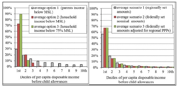
Figure 3 shows the share of spending which accrues to each income decile under various eligibility conditions (left figure) and under various benefit amounts (right figure). These are design effects, which remain the same whether we are looking at the current budget or the increased budget of child allowances. Under the current income test (option 1) only 29% of total spending goes to the poorest income decile. The adjusted income test brings about a higher share of expenditure to the poorest groups of the population. The share of the first decile in total spending rises to 65 and 82% in options 2 and 3, respectively. As far as the benefit amounts are concerned, the distribution of spending becomes more beneficial for the poorest households if the amounts are set at the federal level: in scenarios 2 and 3 over 67% of spending accrues to the bottom decile, while under current design (scenario 1) the share of the bottom decile is 57%.

Distribution of the total spending on child allowances in the simulated reforms under the current budget, 2010.
Source: Own calculations based on RUSMOD.
To sum up, there are strong arguments in favour of bringing the program of child allowances back under the control of federal authorities. It appears to be both politically feasible (before 2005 the program was the federal mandate) and socially just. Currently, the disparity in amounts of child allowances across regions undermines the principles of social justice. In this respect the best available option is to set benefit amounts at the national level, adjusting for regional differences in price levels. To achieve the best results in terms of poverty reduction the unification of standards across regions should be reinforced by bringing the eligibility conditions for child allowances in line with other means-tested programs, i.e. by reducing the number of beneficiaries to those with household income below the poverty line. Even more substantial improvements in all poverty indicators could be achieved by redirecting the resources from the non-poor recipients of housing subsidies to poor households with children.
Having said that, it is important to remind that being purely arithmetical our simulations capture only the first-order consequences of various options of the social assistance reform. Possibly, if we were able to take into account the behavioral response, the advantages of a choice in favor of more targeting would be less evident. The evidence from application of means-tested programs in OECD countries demonstrates that although they demand less resources than universal programs, they are characterized by a number of problems (e.g. produce errors of inclusion and exclusion, require high administrative expenditure, hinder social cohesion, decrease incentives to work, etc. (Oorschot Van 2002). The other consideration that should not be ignored is a tradeoff between the degree of low-income targeting and the size of redistributive budgets. Targeting and budgets are not independent: the budget tend to decrease while targeting increases, as the average voter is less inclined to support the programs from which they do not have any benefit (Pritchett 2005).
6. Concluding remarks
This paper is aimed at documenting the development of RUSMOD – the first full-scale tax-benefit microsimulation model for Russia. The model brings about opportunities of ex ante and ex post assessment of various reforms aimed at improving the Russian tax-benefit system which has a low redistributive effect. Arguably the capacities for poverty reduction in Russia have been exhausted. It is unlikely that a large-scale poverty reduction could be achieved without the reforms that would combine a significant increase in spending on anti-poverty programs with structural changes to provide a more equal access to social programs for households living in different regions of the country.
In order to provide an application of RUSMOD, this paper has assessed the current performance of three means-tested programs and offered several hypothetical reforms that could increase their efficiency, focusing mainly on child allowances. Russia allocates little to anti-poverty programs, and even less resources is reaching the poor because of a low targeting accuracy. Non-poor households constitute more than a half of the beneficiaries of means-tested programs. Such a high rate of leakage is determined by differences in the eligibility rules of the programs, lack of reliable income control procedures and wide occurrence of informal income. The re-allocation of these resources in favour of the poor could bring about significant improvements in the overall and child poverty indicators, as demonstrated by our simulations. This can be achieved by: (1) redistributing resources of each program, within the existing budget, in favor of the poorest households; (2) changing the direction of the budgetary expenditure allocated for social safety nets from programs designed to provide social security to middle income groups, such as housing subsidies, to programs where the main target group are the poor (child allowances). Both measures are not mutually exclusive.
Contrary to the general expectations, the transfer of responsibilities to regions did not help improve the performance of means-tested programs in Russia. Few regions introduced improvements in the way means-tested programs are designed. However, these are not adopted by other regions because there is no authority ensuring that ‘best practices’ are transferred across the regions. Arguably, the federal authorities are best placed to initiate and implement this kind of reform. The simulations show that, holding the current budget constant, by far the greatest reduction in all poverty indicators is achieved if the benefit amounts are set at the national level and adjusted for regional differences in price levels. Hence, there is a strong case for returning the program of child allowances back under the control of federal authorities or developing a strong redistribution mechanism at the federal level to help the poorest regions provide an adequate level of cash support for their poor.
The scope of model applications is not limited to the kind of analysis presented in the paper. For example, one major aspect is investigating the distributional implications of non-cash household income arising from provision of in-kind benefits and public services in Russia. In addition, being compatible with EUROMOD – the Russian model can be used for cross-country policy learning. It means that family benefits of a ‘donor’ country may be integrated into the Russian tax-benefit system and vice versa. Finally, the output of the model can be incorporated into a dynamic model framework in order to study the effects of policy reforms in a longer time perspective, e.g. effects on labour supply or demographic behaviour of households. This is left for future research.
Footnotes
1.
RUSMOD has been constructed using EUROMOD version F5.37 as a platform. EUROMOD is continually being improved and updated and the results presented here represent the best available at the time of writing. Any remaining errors, results produced, interpretations or views presented are the author’s responsibility.
2.
The privileges are not means-tested benefits in the form of cash transfers or free services or discounts on payment for services, provided to vulnerable categories of the population, such as people with disabilities, war veterans, dependents of war victims, victims of the Chernobyl accident, etc., but they also cover numerous categories for services to the state and those based on the occupational status.
3.
In 2010 the US spent 19.9%; the EU countries with their strong emphasis on social welfare spent over 25% (OECD iLibrary, extracted on March 10, 2013).
4.
Poverty headcount is the share of population with per capita income below the cost of the Subsistence Minimum Level (SML) – a cash amount that is necessary to buy a minimum consumer basket of goods and services in order to maintain a person’s health and vital activity.
5.
FP6 Specific Targeted Research Project on ‘Accurate Income measurement for the Assessment of Public Policies’ (AIM-AP). See: https://www.iser.essex.ac.uk/euromod/research-and-policy-analysis-using-euromod/aim-ap
6.
For detailed documentation see: http://www.hse.ru/en/rlms/
7.
The amount of undeclared earnings is computed as the sum of two components: the volume of sales by the population of goods on the markets and the volume of services rendered by individuals.
8.
The computation of taxes and SIC required gross earnings. Since those were not collected in the survey, they were imputed and added to net after-tax income. The imputation of gross income was carried out according to the inversion of rules (Immervoll & O’Donoghue 2001). Inversion is rather straightforward due to the fact that Russia has a constant marginal tax rate and standard tax allowances.
9.
Here we describe the best calibration scenario. In total 8 simulation scenarios based on various combinations of imputation methods were tested. For detailed documentation see: Popova (2012).
10.
Total household consumption is the sum of food items, nonfood items and services, consumer durables and housing. The food component includes the value of food produced at home or received as gift or in-kind payment; non-food and housing components include the value of in-kind subsidies received by privileged or poor households. To arrive at this aggregate, we used the data on individual items, adjusted them from the recall period to a monthly figure, and cleaned the data for implausibly large values (outliers).
11.
The means test for child allowances does not account for the household income. Only earnings or replacement incomes (pensions, maternity allowances, etc.) of parents have to be reported.
12.
Non-take up here means that some of those who are entitled to a benefit are not receiving it. Non-take up rate is defined as the ratio between those who are eligible, but not receiving the benefit, and all those who are eligible.
13.
It means that even if the exact amounts are explicitly set in the regional legislation, the final decisions about the allocation and size of the allowance are made by the local Social protection offices.
14.
Take up probabilities are defined in each relevant policy sheet at the end of the simulation. A user can change these probabilities or switch off the take up correction for each benefit separately by modifying the relevant parameters in each policy sheet.
15.
The average benefit amounts were computed by dividing the total spending on child allowances by the number of recipients, separately for each of the five main categories of beneficiaries (two-parent families, lone mothers, families with 3+ children, disabled children and children of disabled parents). These amounts were adjusted (scaled up or down) to achieve the budget neutrality in each of the scenarios.
16.
The adjustment coefficient is computed as the ratio of the cost of the regional poverty line and the national poverty line.
References
-
1
From child welfare to child well-being. Children’s well-being: indicators and researchAn international perspective on child benefit packages, (Ed.), From child welfare to child well-being. Children’s well-being: indicators and research, Dordrecht, Springer Netherlands.
-
2
Welfare state developments in the Russian Federation: oil-led social policy and the ‘Russian miracle’Social Policy and Administration 43:105–120.
-
3
Post-communist welfare states: reform politics in Russia and Eastern EuropeNew York and London: Cornell University Press.
-
4
The analysis of household surveys: a microeconometric approach to development policyBaltimore, MD: Johns Hopkins University Press.
- 5
-
6
Child benefit and child poverty. CEFIR Working Paper No. WP/00/03Child benefit and child poverty. CEFIR Working Paper No. WP/00/03.
-
7
Comparative EU statistics on income and living conditions: issues and challenges. Eurostat Methodologies and Working PapersLuxembourg: European Communities.
-
8
Measuring the size and impact of public cash support fro children in cross-national perspectiveSocial Science Computer Review 29:85–102.
-
9
Labour market adjustment: is Russia different?. IZA Discussion Paper No. 5588Labour market adjustment: is Russia different?. IZA Discussion Paper No. 5588.
-
10
Inequality and volatility moderation in Russia: evidence from micro-level panel data on consumption and incomeReview of Economic Dynamics 13:209–237.
-
11
Take-up of welfare benefits in OECD countries: a review of the evidence. OECD Social, Employment and Migration Working Papers No. 17Take-up of welfare benefits in OECD countries: a review of the evidence. OECD Social, Employment and Migration Working Papers No. 17.
- 12
-
13
The Distributional Effects of Government Spending and TaxationHousehold incomes and redistribution in the European Union: Quantifying the equalising properties of taxes and benefits, (Ed.), The Distributional Effects of Government Spending and Taxation, Palgrave Macmillan.
-
14
Imputation of gross amounts from net incomes in household surveys. An application using EUROMOD. EUROMOD Working Paper No. EM1/01Imputation of gross amounts from net incomes in household surveys. An application using EUROMOD. EUROMOD Working Paper No. EM1/01.
-
15
Towards a multi-purpose framework for tax-benefit microsimulation: lessons from EUROMODThe International Journal of Microsimulation 2:43–54.
-
16
A short introduction to EUROMOD: an integrated European tax-benefit modelResearch in Labor Economics 25:1–26.
- 17
-
18
Size matters: targeting efficiency and poverty reduction effects of means-tested and universal child benefits in RussiaJournal of European Social Policy 18:260–274.
- 19
-
20
World Poverty: New Policies to Defeat an Old EnemyTargeting welfare: on the functions and dysfunctions of means testing in social policy, (Eds.), World Poverty: New Policies to Defeat an Old Enemy, London, Policy Press.
- 21
-
22
New measures supporting families with children: encouragement of the birthrate or improvement of the living standards? An analysis of the maternity and child support measures introduced in 2007 in the Russian FederationMoscow: UNICEF.
-
23
Poverty and inequality in Russia: sensitivity of poverty and inequality statistics to alternative definitions of households welfare. Illustration using the NOBUS surveyMoscow: The World Bank.
-
24
Constructing the tax-benefit microsimulation model for Russia - RUSMOD. EUROMOD Working Paper No. EM7/12Constructing the tax-benefit microsimulation model for Russia - RUSMOD. EUROMOD Working Paper No. EM7/12.
-
25
The political economy of targeted safety nets. Social Protection Discussion Paper Series No. 0501Washington DC: The World Bank.
-
26
Poverty comparisons: a guide to concepts and methods. Living Standards Measurement Study Working Paper No. 88Washington DC: The World Bank.
-
27
Child well-being in Central and Eastern European Countries (CEE) and the Commonwealth of Independent States (CIS)Child Indicators Research 1:211–250.
-
28
EUROMOD: an integrated Europan benefit-tax model. EUROMOD Working Paper No. EM9/01EUROMOD: an integrated Europan benefit-tax model. EUROMOD Working Paper No. EM9/01.
-
29
EUROMOD: the European Union tax-benefit microsimulation modelThe International Journal of Microsimulation 6:4–26.
-
30
Improving the capacity and usability of EUROMOD – Final report. EUROMOD Working Paper No. EM4/08Improving the capacity and usability of EUROMOD – Final report. EUROMOD Working Paper No. EM4/08.
-
31
Social policy in a cold climate: health and social welfare in RussiaSocial Policy and Administration 40:88–103.
-
32
Human Development Report for the Russian Federation. Modernisation and human developmentMoscow: UNDP.
-
33
Child poverty in rich countries. Report Card No. 6Florence: UNICEF Innocenti Research Centre.
-
34
An overview of child well-being in rich countries. Report Card No. 7Florence: UNICEF Innocenti Research Centre.
-
35
The situation analysis of children in the Russian Federation: on the way to the equal opportunity societyMoscow: UNICEF.
-
36
Microsimulation analysis of the consequencies of monetization of social benefits in Russia. New Economic School Working Paper #WP/2006/063Microsimulation analysis of the consequencies of monetization of social benefits in Russia. New Economic School Working Paper #WP/2006/063.
-
37
Levels and patterns of safely net spending in developing and transition countries. Social Protection Discussion Paper No. 0817Washington DC: The World Bank.
-
38
Adapting EUROMOD for use in a developing country – the case of South Africa and SAMOD. EUROMOD Working Paper No. EM5/09Adapting EUROMOD for use in a developing country – the case of South Africa and SAMOD. EUROMOD Working Paper No. EM5/09.
-
39
First Serbian Tax-Benefit Microsimulation Model - SRMODThe Quarterly Monitor of Economic Trends and Policies in Serbia, 20.
Article and author information
Author details
Acknowledgements
I would like to thank the editors Francesco Figari and Iva Tasseva and an anonymous referee for their helpful comments on this paper and all the members of EUROMOD team at the Institute for Social and Economic Research at the University of Essex for their advice throughout the process of model development. The views expressed are those of the author. I am the only responsible for any errors as well.
Publication history
- Version of Record published: April 30, 2013 (version 1)
Copyright
© 2013, Popova
This article is distributed under the terms of the Creative Commons Attribution License, which permits unrestricted use and redistribution provided that the original author and source are credited.