Modelling the impact of declining Australian terms of trade on the spatial distribution of income
- Institute for Governance and Policy Analysis, University of Canberra, Australia
- University of Canberra, Australia
Abstract
Macroeconomic shocks such as movements in exchange rates or the terms of trade not only affect the overall economy but also affect different areas in a country in different ways, thus creating a spatial distribution of the shock. The effect on some regions is often larger than the national effect as regions differ in terms of resource endowments, economic activities, physical and human capital. The standard national CGE-Microsimulation framework is a useful approach to capture the distributional impacts of macro shocks on households at national and state and territory levels. However, the CGE-Microsimulation framework does not capture the distributional impact of a policy change or an external shock on small geographical areas of interest. To overcome this limitation, this paper extends the framework by linking a spatial microsimulation model to the national CGE-microsimulation framework in a top-down manner to capture the distribution of income in small areas of a macro shock. We simulate a potential decline in Australian terms of trade over 2012–13 to 2017–18 and find significant differences in the spatial distribution of the impacts of the shock.
1. Introduction
The movements in terms of trade (ratio of export to import prices) directly affects a country’s trade activity, which then has implications for growth and income distributions. There is a large and growing literature on the relationship between trade, growth, income distribution and poverty. Berg and Krueger (2003) and Santos-Paulino (2012) provide a useful survey of this literature. Richardson (1995) explores the relationship between trade openness and income inequality. Another related strand of literature focuses on the regional impacts of trade policy (such as trade liberalisation) and shocks (such as movements in terms of trade and foreign demand). For instance, the World Bank (2008) notes the increasing trade activity of a country may lead to higher regional disparities within the country as the areas that have access to ports take advantage of the increased trade.
This is contrary to classical economic theory that states that perfect mobility equalises the economic growth across regions. Henderson (1982) points out that the equalisation mechanism depends on the relative endowment and capacity of different regions in the economy. This argument is supported by Krugman and Livas Elizondo (1996). While a review of the literature by Brulhart (2011) argues that this conclusion may have been too strong, the empirical work by Ezcurra and Rodriguez-Pose (2013) confirms this different spatial effect of trade. In the case of Australia, Behrens et al. (2007) find that the positive impact of trade can be hampered by relatively higher transport costs in mainland rural areas of Australia. Furthermore, greater openness in trade (i.e. the ease of the flow of factors of production and technology in and out of a country) may impact not only on income inequality but also asset inequalities, spatial inequalities, and gender inequalities (Anderson 2005).
Most of the studies on the impacts of trade on inequality and poverty have focused on developing countries (see for instance Kanbur and Venables (2005) for a collection of articles). However, the spatial distribution of a decline in terms of trade in a developed country like Australia is of interest, given the importance of the income gains of the recent boom in terms of trade (largely on the back of a resources boom).
The spatial impacts of these macro shocks such as a decline in terms of trade may be important for a number of reasons. Parliamentary representatives elected from regions for State and Federal governments often demand regional detail in economic and social analysis. Policy makers concerned with regional disparities in employment, income and overall economic opportunities demand detailed regional results, in particular for economic and social impacts on the households and the communities in small areas (Horridge et al., 2005). Other stakeholders (such as unions, NGOs, local community groups and other interest groups) who work with and represent small regions are also interested in the impacts of macro-economic change on their region. Local and regional issues are also important to academics, researchers and modellers who have a responsibility to provide independent analysis to inform policy development that may include the likely impact of a policy or an external shock on local communities.
Before the onset of the Global Financial Crisis (GFC), the Australian terms of trade had been on a rising trend for over a decade (Jaaskela & Smith 2013 and see Figure 1). The authors of this paper find that higher terms of trade tend be expansionary but not inflationary. It is worth noting that unlike previous booms in Australian terms of trade such as in the 1920s and 1950s, which were followed by falling output and increased unemployment, the recent increases in the terms of trade created less instability (Battellino, 2010). Gregory points out that the boom in the terms of trade in the last decade or so has raised the average living standards in Australia to above that of US (Gregory, 2012).
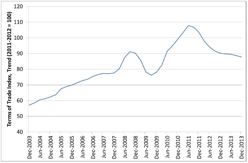
Movements in Australian terms of trade.
Source: ABS.
Although the Australian terms of trade declined slightly during the GFC, the terms of trade was back to an increasing trend a year after the onset of GFC. However, it has now shown a steady decline since mid-2011 (see Figure 1). Given the benefit that the Australian economy experienced from rising terms of trade, there are concerns that the downward trend could not only harm the economy but also change the income distribution among households in different locations in Australia. It is thus vital that the spatial effects of a steady decline in terms of trade be examined in greater detail.
In this paper, we use a computable general equilibrium (CGE) model, a national microsimulation model and a spatial microsimulation model to capture the impact of a macro shock on the distribution of income in small regional areas of the Australian economy. It is important to note that the standard Computable General Equilibrium (CGE) models do not capture the distributional impact of a policy change or an external shock in small geographical areas. To overcome this limitation, we have sequentially linked a CGE, a microsimulation and a spatial microsimulation model in a top-down manner to capture the distribution of income in small areas. How the models are sequentially linked, including how consistency between the models has been achieved, and the transmission of a macro shock from the macro and sectoral impacts to its distributional impacts in the small geographical regions, is the focus of the paper. To implement the framework we simulate a potential Australian terms of trade decline over a five year period (2012–13 to 2017–18).
With this background, the rest of the paper is organised as follows. The next section describes the modelling framework. Section 3 explains how the terms of trade shock is modelled. Section 4 discusses the results and Section 5 concludes.
2. The framework: CGE-microsimulation linkages
Before developing a model which brings together a number of other models, it is useful to specify an approach that will link the different models. This paper uses the framework developed by Rao et al. (2013) that links a CGE model with a microsimulation and spatial microsimulation model. This link is achieved by linking the CGE output to different types of households through the household members that work in different industries and occupations. Based on these different types of households, this method simulates how tax payments and transfer payments respond to the macro-economic shock provided in the CGE model. The spatial effect is then estimated by distributing the households into small areas using a spatial microsimulation model.
Figure 2 depicts the modelling approach used to simulate the distributional impacts of an Australian terms of trade decline on the Australian and regional households. The terms of trade shock is a macro shock and its economy-wide impacts can be best captured by a computable general equilibrium model as shown by link 1 in Figure 2. We use the ORANI CGE model of the Australian economy (Dixon, et al., 1982) with an extended forecasting feature. The extended model with the forecasting feature is described in detail in Rao (2011). The output of interest of the CGE model is the changes in the employment by industry and occupation resulting of the terms of trade shock (link 2 in Figure 2), which captures the winners and losers in terms of industries and occupations at the national level.
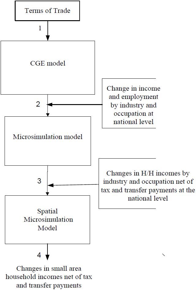
The modelling framework.
Most national CGE models provide a relatively disaggregated (sectors, occupations, skills/qualifications) representation of the economy. However, traditionally, one or a relatively small number of representative (homogenous) household groups describe the income distribution in most CGE models, and thus do not capture the heterogeneity of households represented in the population (Colombo, 2010). Moreover, CGE models typically do not include complex tax and transfer payment systems present in developed countries like Australia and therefore cannot capture the full impact of a policy or external shock net of tax and transfer payments. For these reasons, CGE models have limited application for distributional analysis.
To capture the full distributional impacts of the TOT shock on households at the national level, including the full application of the Australian tax and transfer payments, we pass the output of the CGE model (changes in factor employment and incomes by industry) to STINMOD – a national tax and transfer microsimulation model of the Australian economy (Lambert, et al. 1994, Percival et al., 2007). STINMOD calculates the distribution of the household income (cross-classified over a number of household characteristics) at the national level (which can be disaggregated into State and Territory levels), after taking into account the tax and transfer payments (link 3 in Figure 2). However, the distribution of household income may not fully represent small geographical areas of interest, given that small areas are not normally captured by national sample surveys on which STINMOD is based. To capture the impacts in small areas we link STINMOD to SpatialMSM, a spatial microsimulation model of the Australian population (Tanton et al., 2011), which derives datasets of small areas using Census data and data from official ABS sample surveys to capture household details in small areas. The output from STINMOD, that is, the distribution of household income at the national or state/territory levels, net of tax and transfer payments, is passed to SpatialMSM to calculate the distribution of household income (cross-classified over a number of household characteristics) in small geographical areas (link 4 in Figure 1).
3. Application of the modelling framework
3.1 The CGE model and the Terms of Trade Shock
The illustrative terms of trade (TOT) shock is an annual decline in the terms of trade of 5 percent over 5 years from 2011–12 to 2016–17. The compounded impact of the shock over 5 years amounts to a decline of 22.6 percent. As mentioned earlier, the macro and the sectoral impacts of the terms of trade shock at the national level is simulated using the ORANI CGE model of the Australian economy. How the TOT shock is implemented is explained with the following stylised equations represented in the ORANI CGE model.
Equation (1) defines the foreign currency price of exports (PX) as negatively related to the volume of exports (X) (implying a downward sloping demand schedule) and positively or negatively related to an export demand shift variable(V), depending on whether the demand schedule shifts outwards (right) or inwards (left) respectively. The bold V in Equation 1 indicates the export shift variable is exogenous in equation 1. Equation (2) defines the TOT as the ratio of foreign currency export prices (PX) to foreign currency import prices(PM). The model assumes that Australia is a price taker in the overseas market (the small country assumption) and therefore takes foreign currency import prices as given or exogenously determined. The bold PM denotes the exogenous nature of the import price in equation (2)1. Given that the foreign currency import price (PM) is fixed in equation (2), TOT is then determined by PX or equation (1). PX in turn is determined by movements in X or V or both.
The TOT is endogenous in Equation 2, largely determined by the foreign currency price of exports, (PX), that is by Equation 1. In order to shock TOT, the variable needs to be moved to the exogenous category by moving a suitable exogenous variable to the endogenous category. The suitable exogenous candidate for the swap is the export shift variable V in equation 1. With the swap, the TOT shock is accommodated by movements in V but the secondary effects of the shock also cause movements in X, as will be explained below. The macro effects of 22.6 percent decline in terms of trade shock is discussed below.
A CGE model of the size of ORANI2 involves many economic relationships defined by many equations and variables in the model. To summarise this detail and elucidate the main features of ORANI, a stylised or back of the envelope (hereafter BOTE) model based on the BOTE models of Dixon and Rimmer (2002) and Giesecke (2008) is developed to explain the macro effects of the policy simulations of a decline in terms of trade. The BOTE model is explained as follows.
The model assumes there is a single domestically produced commodity, which is used both domestically and exported, and a single imported commodity. The BOTE model is represented in Equations 3-14 (below) and is interpreted as follows. Equation 3 is the GDP identity in constant prices, which is the sum of all final demands: real private consumption, real public consumption, real investment and net exports. 4 describes an economy-wide constant returns to scale production function, relating GDP to inputs of labour (L), capital (K) and technology (A). 5 defines real private and real public consumption as a proportion of real Gross National Product (GNP) via average propensity to consume (APC). 6 defines the ratio of real private consumption to real public consumption. 7 relates GNP to GDP multiplied by a positive function of the terms of trade (TOT) less interest payments on net foreign liabilities (R). 8 defines net foreign liability (NFL) as a positive function of K and APC and a negative function of GNP. More specifically, 8 relates changes in NFL to movements in savings and investment gap over the simulation period.
Equation 9 relates imports positively to GDP and TOT. 10 defines the foreign currency price of exports (PX) as negatively related to the volume of exports (X) (implying a downward sloping foreign export demand schedule) and positively related to an export demand shift variable (V).
TOT is defined by 11 as the ratio of foreign currency export prices (PX) to import prices (PM). 12 defines the aggregate investment/capital ratio (Ψ), which reflects business confidence in ORANI and therefore determined exogenously. The constant returns to scale production function implies homogeneity of degree one in K and L, and thus, the marginal product functions can be expressed as functions of K/L and A. Hence 13 shows that the profit maximising capital labour ratio, K/L is positively related to A and TOT but negatively related to the rate of return (ROR). Finally, 14 positively relates the real wage to K/L, A, and TOT.
3.2 Microsimulation models and links to CGE
As mentioned above, this study uses two types of microsimulation model to estimate the spatial impacts of the decline in terms of trade. The first microsimulation model is STINMOD, which is a static (and non-behavioural) federal tax and transfer payments model of the Australian economy. STINMOD estimates the changes in household income and federal tax and transfer payments for each different household observed in the microdata (Lambert et al. 1994). STINMOD therefore has two important components: a database and the Tax and Transfer rules of the Commonwealth of Australia. The STINMOD database is based on the national Income and Housing and Household Expenditure Survey (but includes data from other sources as well). The database used in this simulation is based on the 2009/2010 survey. The Tax and Transfer rules of the Commonwealth (which largely changes with each annual budget announcement of the Commonwealth) is applied to the unit data in the database to assess the tax-transfer payments to different types of households represented nationally.
However, each unit record in STINMOD represents a person observed in the micro data, whereas the tax and transfer payments are largely based on the total household income. A household identifier in the database assigns the person to a unique household. This is an important feature of this database that allows us to connect the results from the CGE model to STINMOD as the person records contain the industry and occupation detail that can be mapped to the industry and occupation dimensions of the CGE model. The household identification will also be important as the tax and transfer are largely calculated based on the characteristics of the household including its income, number of dependents and the type of tenure arrangements of the households. Passing the output of the ORANI CGE model, namely the employment and wages by industry and occupation – the linking aggregate variables (LAVs) – to STINMOD, we achieve two outcomes. First, STINMOD takes movements in industry by occupation employment and wages from the CGE model and distributes them across the persons belonging to respective household types represented at the national level. Second, STINMOD calculates the movements in household income (cross-classified across a number of household characteristics) after taking into account the tax and transfer payment rules applicable to each household type represented in the total population.
The linking of the ORANI CGE model and STINMOD proceeds in two steps. In the first step, STINMOD simulates a baseline forecast of industry employment (occupation) and wages using initial weights (weights of each household type in the total population) generated by STINMOD based on the demographic forecasts to ensure that each household type is properly represented in the sample in the forecast period.
In the second step, STINMOD accommodates the movements in industry employment and wages (LAVs) from the CGE model resulting from the terms of trade shock. This is akin to a policy simulation in STINMOD of the terms of trade shock. A reweighting approach is used to accommodate the movements in industry employment by occupation passed down by the CGE model. The reweighting method used here is called GREGWT developed by the Australian Bureau of Statistics (ABS) (Bell, 2000) and is based on a generalized regression method of Singh and Mohl (1996). Buddelmeyer et al. (2012) uses a similar approach to analyse the forecast distributive impacts of climatic change in Australia. One important aspect of this reweighting process is the benchmark table (Table 1). This table contains critical information on household/individual characteristics such as age, education, occupation and household type represented in the population. In this simulation, STINMOD takes the changes in employment passed down by the CGE model by changing the number or proportion of workers in every industry and occupation, while ensuring that the other characteristics such as age and education structure remain unchanged.
Employment simulation benchmark tables.
| Number | Benchmark |
|---|---|
| 1 | Number of Persons aged 15+ |
| 2 | Occupation of Reference Person by Industry of employment |
| 3 | Occupation of Spouse by Industry of employment |
| 4 | Age of Reference person by Age of Spouse by family type |
| 5 | Non School Qualification (reference person and Spouse) and Number of Dependents |
-
Source: ABS Census of Population and Housing, 2011.
With regards to the changes in wages from the CGE model, STINMOD distributes the movements in wages (by industry and occupation) as follows.
where is the base period income (STINMOD database) of a person (p) belonging to a household (h), working in industry (i) in occupation(o); is movements in wages by industry and occupation, which is the output of the CGE model from the decline in the terms of trade; and is the new income of the same person who belongs to the same household, same industry and same occupation. That is, equation 15 is an updating equation that updates the individual’s income after taking into account the changes in income as the result of the structural changes in the economy caused by the terms of trade decline.
With the total income of each household computed in Equation 16, we can now apply the tax and transfer rules to compute the final impact of the decline in terms of trade on each household type at the national level. The disposal income of household h (DIh) is given by
and
where Transferh and Taxh corresponds to the transfer payments and taxes applicable to household h’s total income after the impact of the decline in the terms of trade has been taken into account. Note that both the tax and transfer payments depend on the level of household income (equations 18 and 19).
3.3 Links to spatial microsimulation model
As mentioned earlier, the focus of the paper is to find the impact of the terms of trade decline in small geographical areas of Australia, not captured by the official sample surveys on which STINMOD’s database is based. These small geographical areas are Statistical Local Areas (SLAs) as defined by the Australian Bureau of Statistics (ABS). In order to find impacts on SLAs, we link the results of STINMOD to SpatialMSM, a spatial microsimulation model of the Australian economy. Spatial microsimulation is a technique used to derive datasets to represent the population in small areas. SpatialMSM is designed to allocate private income, tax paid and transfer received for each person on the database, as well as the changes in the weights that capture the employment impact, to the small areas – the SLAs in Australia. The SpatialMSM microsimulation model uses a reweighting procedure to reweight the micro data set of STINMOD to the Census benchmarks for each SLA, thus creating a synthetic household dataset for each of them. This dataset is then used to generate household characteristics of interest to analyse the distributional impacts of a policy change on a small area (Harding et al. 2009, Tanton et al. 2009), such as an SLA.
To enable the spatial microsimulation model to capture both the impact from the CGE model and STINMOD, the reweighting process has to constrain to the benchmarks containing the main linking variable from CGE and STINMOD (listed in Table 2). The main linking variable of the CGE output is the changes in wages and employment by industry and occupation. Therefore, the first three benchmarks in Table 2 – age by sex by labour force status, non-school qualification and industry and occupation – are chosen to accurately capture the movements in the industry and occupation in the baseline. The next four benchmarks are introduced to ensure that the STINMOD results are applicable to different areas as these four benchmarks contain the main variables that could affect the amount of tax and transfer received by different households.
Census benchmark tables to generate dataset for small areas.
| Number | Benchmark |
|---|---|
| 1 | Age by sex by labour force status |
| 2 | Non-school qualification |
| 3 | Industry and Occupation |
| 4 | Household type |
| 5 | Number of persons usually resident in household |
| 6 | Tenure type by weekly household income |
| 7 | Dwelling structure by household family composition |
-
Source: ABS Census of Population and Housing, 2011.
The reweighting procedure is an iterative process and will stop when the new weights produce estimates that are close to the benchmarks, that is, convergence is achieved. There may be cases where convergence is not achievable, and in these cases we need to stop the procedure when a specified maximum number of iterations has been reached. In this case, the model reports a non-convergence error. This reported error is then used to test the accuracy of the model and those areas that do not converge are excluded from the small area statistics produced. We find that 229 of the 1392 SLAs are to be excluded from further analysis since the process could not produce a reasonable solution for them (non-convergence). Most of these areas are remote areas with low population. This creates a baseline dataset for 1163 SLAs.
Note we have already computed the household income net of tax and transfer payments as a result of the terms of trade decline for each observation using STINMOD. We apply this result (income net of tax and transfer payments) to each observation in each SLAs. This results in new household disposal income for all SLAs in the data set, which reflects the decline in the terms of trade impacts.
4. Results and discussion
Table 3 reports the macro results of the terms of trade shock. We use the BOTE model described above to explain these macro effects. Bold letters in the BOTE model indicates that the variables are exogenously determined in the policy simulation. Note that Equations (1) and (2) are reproduced in the BOTE model as Equations 10 and 11 for easy reference. As explained earlier, the source of the terms of trade shock is a fall in the foreign demand for Australian exports. In terms of the BOTE model, there is a negative shock to TOT in Equation 10 causing a leftward shift in the export demand schedule (a negative movement in V) inducing declines in both foreign currency price of exports (PX) and the volume of exports (X). The fall in PX induces the fall in TOT via equation 11. The effects of the fall in TOT of 22.6 percent (row 18, Table 3) are traced as follows.
Policy simulation: A terms of trade decline of 22.6 percent (5% pa) over the 5 years from 2011–12 to 2016–17 – the percentage deviations in macro variables from the baseline forecasts.
| Macro variables | Deviations from forecast values | |
|---|---|---|
| 1 | Real GDP | −0.64 |
| 2 | Real GNE | −2.38 |
| 3 | Real GNP | −3.66 |
| 4 | Total factor productivity | 0.00 |
| 5 | Average Propensity to Consume | 0.00 |
| 6 | Real private consumption | −2.33 |
| 7 | Real public consumption | −2.33 |
| 8 | Real investment | −2.56 |
| 9 | Real exports | 2.65 |
| 10 | Real imports | −8.06 |
| 11 | Employment (hours weighted) | 0.00 |
| 12 | Employment (wage weighted) | 0.07 |
| 13 | Capital Stocks | −2.29 |
| 14 | Real wage | −8.93 |
| 15 | Nominal exchange rate | 30.23 |
| 16 | Real exchange rate | −37.91 |
| 17 | Terms of trade | −22.60 |
| 18 | Consumer price index | 0.00 |
| 19 | Price deflator for GDP | −5.52 |
| 20 | Price deflator for investment | −0.40 |
| 21 | Price deflator for consumption | −1.37 |
| 22 | Change in the ratio of balance of trade to GDP | 0.03 |
| 23 | Change in the ratio of net foreign liabilities to GDP | −0.69 |
Given that L, ROR and A fixed in Equation 4, the decline in TOT will cause a decline in K (row 13), since K is positively related to TOT. With A and L exogenous in Equation (4), the decline in K will cause real GDP to fall (row 1). The declines in GDP and TOT cause GNP to decline (row 3) via Equation 7. The decline in GNP, with APC and Γ fixed causes both private and public consumption to fall via Equations 5 and 6 (rows 6 and 7) respectively.
Given that L, ROR and A are fixed in Equation 4, the decline in TOT will cause a decline in K (row 13), since K is positively related to TOT. With A and L exogenous in Equation (4), the decline in K will cause real GDP to fall (row 1). The declines in GDP and TOT cause GNP to decline (row 3) via Equation 7. The decline in GNP, with APC and Γ fixed causes both private and public consumption to fall via Equations 5 and 6 (rows 6 and 7) respectively. A decline in K with Ψ exogenous implies a fall in investment (I) via Equation 12 (row 8). With C, G and I determined, so is absorption or GNE (row 2). Note that GNE declines faster than GDP, which via Equation 3, implies that the trade balance (X-M) must move towards surplus (row 22). Thus, imports decline (row 10) and exports increase (row 9), facilitated by a real exchange rate depreciation (row 16). The decline in imports is explained by the BOTE Equation 9, that is, the declines in GDP and TOT both cause imports to fall, given that both GDP and TOT are positively related to GDP. Equation 14 shows that the declines in K and TOT, with A fixed causes the economy-wide wage rate (W) to fall, which will have significant implications for spatial distribution of employment and income discussed later in this paper.
4.1 The Sectoral and Employment Effects
The sectoral impacts of the TOT decline can be explained from the macro impacts. Table 4 shows the movements in sectoral output, employment and wage rates. Macro results show exports increase facilitated by exchange rate depreciation. This is reflected in an increase in the output of export-oriented sectors (sectors 1–3) in Table 4. The output of transport and storage (sector 9) also increases given that this sector supports export sectors. The decline in overall investment is reflected in the decline in the output of the construction sector (sector 5). The decline in consumption is reflected in the decline in output of sectors largely producing for the domestic market, the remaining the sectors in Table 4. However, the sector such as accommodation, cafes & restaurants (sector 8), which supports tourism (the sector that benefits from exchange rate depreciation) and the education sector (sector 16), which has a significant export component show relatively small declines in output.
Movements in sectoral output and employment.
| Sector | Input (1) | Employment (2) | Wage rates (3) | |
|---|---|---|---|---|
| 1 | Agriculture, Fisheries & Forestry | 1.88 | 3.40 | −1.32 |
| 2 | Mining | 4.13 | 7.25 | −7.31 |
| 3 | Manufacturing | 2.71 | 4.47 | −5.84 |
| 4 | Electricity, Gas & Water | −0.30 | 1.89 | −8.59 |
| 5 | Construction | −2.20 | −1.76 | −10.75 |
| 6 | Wholesale Trade | −2.40 | −1.86 | −8.93 |
| 7 | Retail Trade | −3.00 | −2.35 | −11.69 |
| 8 | Accommodation, Cafes & Restaurants | −0.01 | 0.78 | −9.83 |
| 9 | Transport & Storage | 0.26 | 0.99 | −8.09 |
| 10 | Communication Services | −1.00 | 1.01 | −8.95 |
| 11 | Finance & Insurance | −0.28 | 0.73 | −7.46 |
| 12 | Property & Business Services | −0.59 | 1.66 | −8.50 |
| 13 | Professional Science & Technical Services | −1.09 | −0.83 | −8.01 |
| 14 | Administrative & Support Services | −0.50 | 0.63 | −8.24 |
| 15 | Public Administration | −2.14 | −1.69 | −8.72 |
| 16 | Education | −0.10 | 0.15 | −9.27 |
| 17 | Health & Social Services | −0.82 | −0.68 | −11.56 |
| 18 | Arts & Recreation | −1.22 | −0.58 | −9.73 |
| 19 | Other Services | −1.04 | −0.35 | −9.65 |
| 20 | Agriculture, Fisheries & Forestry | 1.88 | 3.40 | −1.32 |
| 21 | Mining | 4.13 | 7.25 | −7.31 |
| 22 | Manufacturing | 2.71 | 4.47 | −5.84 |
| 23 | Electricity, Gas & Water | −0.30 | 1.89 | −8.59 |
Movements in employment follow movements in output, given that employment and output are positively related. This holds for all sectors except for sectors 4, 8, 10 and 16, where decline in output is accompanied by increases in employment. An explanation for this is that as workers move or are reallocated between sectors, some sectors that experience declines in output would tend to hire more quantities of cheaper workers to minimise costs. The relationships between the movements in employment (column 2) and wage rates (column 3) in Table 4, as the result of movements of labour between sectors are explained as follows.
The expansion of export-oriented sectors attracts labour, thus increasing the supply of labour to these sectors, causing employment to increase and wage rates to fall (sectors 1–3, and 9). Sectors that experience a decrease in output induces a fall in demand for labour, reflected in the fall in employment and wage rates (sectors 5–7, 13, 15 and 17–19). Sectors which experience declines in output but increases in employment and falling wage rates reflect workers offering labour at lower rates to remain employed (sectors 4, 8, 10–12, 14 and 16).
The analysis shows that the decline in the terms of trade simulation induces significant changes in the composition of output, and thus a reallocation of labour between industries. What is also significant is that the decline in terms of trade causes wage rates to fall across all the sectors and will have implications for changes in the spatial distribution of income. To capture the spatial distribution of income across households the output of the CGE model, namely the movements in employment and wages by sectors is passed to microsimulation models.
4.2 The effects of the tax and transfer system
Table 5 shows how at the national level the tax-transfer system has reduced the overall impact of the decline of the TOT on the income changes. The tax paid will be lower and transfers will be higher and in this particular exercise the fall in the tax paid seems to be more dominant than the increased transfer that the government needs to pay to the household. The model is also able to separate the impact of the employment effect and the wages effect. The changes in the employment composition due to the drop in the TOT may actually increase the overall income. However, the impact is very small while the negative impact from the decrease in wages per person in different industry and occupation is much higher. This means that the current employment levels could realistically be retained only if employees were willing to take a wage cut. The CGE result also indicates that workers in construction, trade and public services (especially public administration and health-social services) may need to find employment outside the sector, as it is likely that these sectors will suffer lower incomes.
National effects from the CGE and microsimulation models.
| Employment effect (%) | Income effect (%) | Total effect (%) | |
|---|---|---|---|
| Private Income | 0.15 | −8.10 | −7.95 |
| Tax paid | 0.12 | −13.47 | −13.35 |
| Government transfer | −0.21 | 1.98 | 1.77 |
| Disposable Income | 0.11 | −5.49 | −5.38 |
The impact on tax paid by the employee is much higher as a proportion than the effect on overall private income. This is due to the progressiveness of Australian tax rates. For example, if the drop in wages made gross wages fall below $80,000 a year then the reduction in tax paid is not only due to the decrease in the taxable income but also the lower rate faced by the tax payer.
The change in the tax paid is even bigger if the annual gross income drops below $37,000, the next tax threshold. On the other hand, the increase in government transfer payments from the drop in TOT is low. This is probably due to the fact that the unemployment rate is assumed to be relatively constant and the income test component of Government transfer payments in Australia has a lower impact than the changes to employment status and family conditions. Therefore, the increase in the Government transfers may not be as crucial as the larger drop in tax in ensuring the disposable income has been less affected by the drop in TOT.
4.3 The regional effects
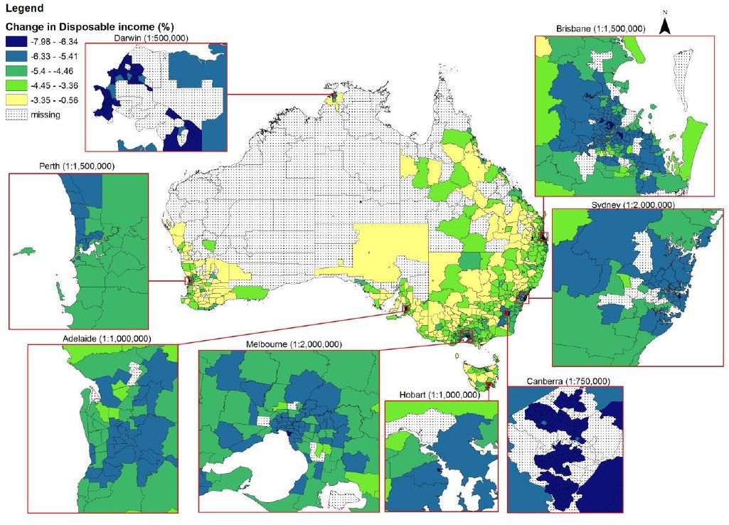
The spatial effect of the TOT shock, estimated using the SpatialMSM model, is shown in Figure 3. This figure depicts the impact in a choropleth map with the darker colour indicating the higher impact. The classification ranges for this map use natural breaks where the different classification is determined by the largest difference between two subsequent changes in the distribution. This classification is often used for identifying clusters as well as separating the relatively high impacts from low ones. The shaded (dotted) areas in the middle of Australia are areas where our spatial microsimulation model was not able to derive estimates due to non-convergence (see above).

Spatial impact on incomes of a change in terms of trade.
Given that the three sectors experiencing the greatest drop in wage rates as a result of the drop in TOT are Retail Trade, Health-Social Services and Construction, we would expect Capital Cities in Australia, where these sectors are larger, to experience a greater impact of the drop in TOT on gross income. The regional effect of the change in the TOT confirms this expectation with a darker colour showing areas with greater decreases. The figure indicates that the greatest decrease in gross income will be in Canberra, Darwin and the areas surrounding Hobart while Sydney, Brisbane, Melbourne, Adelaide and Perth experience a lower decrease. In Perth, the impact is estimated to be mainly in the North part of the city. In contrast, the impact on Canberra seems to be spread around the surrounding areas from where commuters that work in Canberra come from.
Besides capital cities, Figure 3 also indicates that the east coast of Australia will experience a considerable impact. This is especially true for the south east coastal area of NSW to Brisbane in Queensland.
The greater impact on the incomes of households in Canberra, Darwin and Hobart does not mean that the tax reduction will come from those cities. The income structure will play an important role in determining the reduction in tax paid. Figure 4 shows that the area surrounding Hobart experiences a higher reduction in tax paid and also identifies areas such as Gosford and the Blue Mountains in the North and West of Sydney, respectively, as having a greater reduction in tax paid than other areas. This is also true for the areas surrounding Melbourne, Brisbane, Adelaide and Canberra. In addition, areas on the South East Coast are estimated as experiencing greater drops in tax paid compared to capital cities. In contrast, areas experiencing a lower reduction in tax paid are relatively wealthy areas such as North Sydney and inner city areas of Melbourne, Brisbane, Canberra and Adelaide. The reduction in tax paid in Perth is estimated to be much lower than other capital cities.
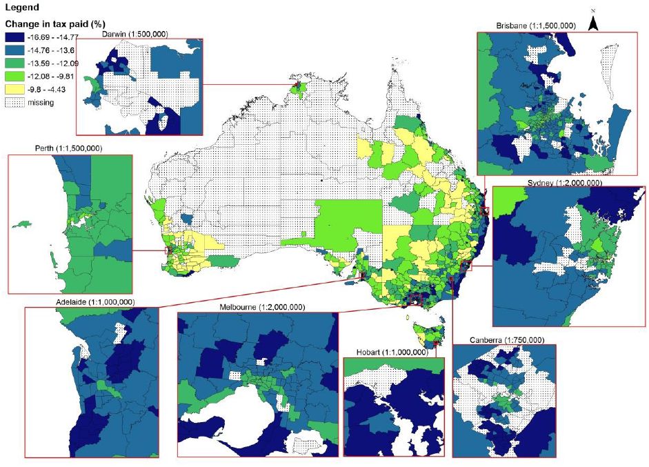

Spatial reduction in tax paid as a result of a change in terms of trade.
The next variable we looked at from the microsimulation models was Government transfer payments (Figure 5). Although the income structure plays a role in Government transfer payments, income is not the only factor determining transfer payments, so changes in Government transfer payments are more likely to be determined by the distribution of different household characteristics among regions in Australia. As a result, our estimation does not indicate a huge difference in changes to Government transfer payments between areas. The relatively higher increase in capital cities is more likely due to the greater fall in the household incomes in those areas. The impact also seems to be spread more evenly around capital cities. There are some suburbs in Melbourne, Brisbane and Canberra that we estimate will receive higher increases in transfer payments. One argument that can be offered for this is the spread of children in these areas. For example, Gungahlin in the North of Canberra and Tuggeranong in the South of Canberra have relatively high increases. Both these are fairly new areas with a higher proportion of young families.
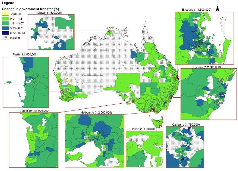

Spatial impact on government transfer payments as a result of a change in terms of trade.
Finally, we look at the changes in disposable income (Figure 6). Disposable income is the amount that is available for households to spend on goods and services, so it takes out tax paid from gross income. One of the advantages of the type of analysis used for this model is that disposable incomes can be calculated from the base dataset. One of the major differences between the change in disposable income compared to the change in gross income is that the East Coast area no longer experiences a large drop in disposable income. This is likely due to the large tax reduction estimated for the area. The estimated tax reduction has also reduced the reduction in incomes in capital cities such as Sydney, Melbourne, Adelaide, Hobart, and to some extent Brisbane and Perth. This means the income fall is mainly concentrated in Canberra and to a lesser extent Darwin.

Spatial impact on disposable income as a result of a change in terms of trade.
5. Conclusion
Macro-economic shocks can have different spatial impacts across the country depending on resource endowments, physical and human capital among other factors. The final impacts on households will depend on the characteristics of each household and the national tax transfer system. In this paper, we combine a CGE, a tax-transfer microsimulation model and a spatial microsimulation to transparently trace the spatial distribution of the impacts of a terms of trade decline.
In particular, we find that capital cities are most affected by a decline in the TOT. The industries most affected are retail, construction and health and social services sectors, all of which are largely located in capital cities. Since the CGE model is linked to a tax/transfer microsimulation model, it enabled us to compute tax paid, Government transfer payments disbursed; and finally disposable income. We find that government transfer payments were not as affected by the TOT decline compared to income and tax paid as these payments are not entirely dependent on incomes. This linking of CGE and microsimulation models is a useful framework, as it is able to show the regional/spatial impacts of a macro-economic policy or external shock that enables policy makers and researchers to identify the areas affected most by such shocks.
The model described in this paper has some limitations. The main limitation is that the model relies on the distribution of income by industry and occupation among household members and small geographic areas to distribute the impact of the TOT decline at a national level. This means that the relationship between economic sectors at the local level is assumed to be in line with the relationship at the national level. This may not always be true as the market behaviour in regional areas can be different to the national market behaviour. In addition, the relationship between different regions has only been captured by the relationship between different industrial sectors. Therefore, the issue of whether market behaviour changes due to clustering of areas within a certain industrial sector has not been assessed by the model.
The other limitation is that the microsimulation model used in this paper is static and only estimates the immediate impact from the decline. Long term estimates of the impact would create some challenges. For example, people in different areas that suffer similar impacts may respond differently as they could have different levels of resilience. Furthermore, the response may affect the CGE modelling, for example, through changes in consumption and this means the model would need some iterative interaction between the CGE and microsimulation model.
In this paper, we have been able to show how a CGE, microsimulation and spatial microsimulation can be linked. While this has been shown in this paper, there is still further development required. Other macro-economic shocks can be modelled, and behavioural responses could be incorporated into the model. Further, the CGE model is still a national model, and assumes national relationships between industries – this assumption could be relaxed using a regional CGE model.
Footnotes
1.
Given that the foreign currency import price is fixed, the movements in the domestic currency import price will reflect movements in the nominal exchange rate.
2.
The database of ORANI used in this simulation has 169 industries and commodities and 81 occupations.
References
-
1
Openness and inequality in developing countries: A review of theory and recent evidenceWorld Development 33:1045–1063.
- 2
-
3
Countries, regions and trade: On the welfare impacts of economic integrationEuropean Economic Review 51:1277–1301.
- 4
-
5
Trade, Growth and Poverty: A Selective Survey. IMF Working PaperWashington, DC: International Monetary Fund.
- 6
-
7
Linking a microsimulation model to a dynamic cge model: Climate change mitigation policies and income distribution in australiaInternational Journal of Microsimulation 5:40–58.
-
8
Linking CGE and Microsimulation Models: A Comparison of Different ApproachesInternational Journal of Microsimulation 3:72–91.
-
9
Contributions to Economic AnalysisContributions to Economic Analysis, 142, North-Holland Publishing Company, Amsterdam.
-
10
Dynamic general equilibrium modelling for forecasting and policy: a practical guide and documentation of MONASHAmsterdam: Elsevier Science B.V.
-
11
Does Economic Globalization affect Regional Inequality? A Cross-country AnalysisWorld Development 52:92–103.
-
12
The effects of recent structural, policy and external shocks to the Australian economy, 1996/97-2001-02. Australian Economic Papers15–37, The effects of recent structural, policy and external shocks to the Australian economy, 1996/97-2001-02. Australian Economic Papers, 47.
-
13
Living standards, terms of trade and foreign ownership: reflections on the Australian mining boomAustralian Journal of Agricultural and Resource Economics 56:171–200.
-
14
Improving work incentives for parents: the national and geographic impact of liberalising the Family Tax Benefit income testThe Economic Record 85:48–58.
-
15
Systems of cities in closed and open economiesRegional Science and Urban Economics 12:325–350.
- 16
-
17
Terms of Trade Shocks: What Are They and What Do They Do?Economic Record 89:145–159.
- 18
- 19
-
20
An introduction to STINMOD: a static microsimulation Model. NATSEM Technical Paper No 1Canberra: University of Canberra.
-
21
STINMOD (static income model) 2007In: A Gupta, A Harding, editors. Modelling our future: population ageing, health and aged care. Amsterdam: Elsevier BV. pp. 477–82.
-
22
A Systems Approach to Analyse the Impacts of Water Policy Reform in the Murray-Darling Basin: a Conceptual and an Analytical Framework. NATSEM Working Paper 2013/22Canberra, Australia: University of Canberra.
-
23
ORANI-ED: A CGE Model of the Australian Economy for Labour Market Forecasting and Education and Training Sector Policy AnalysisORANI-ED: A CGE Model of the Australian Economy for Labour Market Forecasting and Education and Training Sector Policy Analysis, Unpublished PhD Thesis, Faculty of Business and Economics, Centre of Policy Studies, Monash University, http://arrow.monash.edu.au/hdl/1959.1/540569.
-
24
Income inequality and trade: how to think, what to concludeJournal of Economic Perspectives 9:33–55.
-
25
Trade, Income Distribution and Poverty in Developing Countries: A survey. Discussion Paper No. 207, UNCTADNew York: United Nations.
-
26
Understanding calibration estimators in survey samplingSurvey Methodology 22:107–115.
-
27
Old, single and poor: using microsimulation and microdata to analyse poverty and the impact of policy change among older AustraliansEconomic Papers: A Journal of Applied Economics and Policy 28:102–120.
-
28
Small area estimation using a reweighting algorithm931–951, Journal of the Royal Statistical Society Series A, (Statistics in Society), 174.
-
29
World development report 2009: Reshaping economic geographyWashington, DC: World Bank.
Article and author information
Author details
Acknowledgements
This research was supported by the Australian Government’s Collaborative Research Networks (CRN) program.
Publication history
- Version of Record published: April 30, 2014 (version 1)
Copyright
© 2014, Vidyattama et al.
This article is distributed under the terms of the Creative Commons Attribution License, which permits unrestricted use and redistribution provided that the original author and source are credited.