A microsimulation model to evaluate Italian households’ financial vulnerability
- Institute Bank of Italy, Financial Stability Directorate, Via Nazionale, Italy
Abstract
We build a microsimulation model to monitor the financial vulnerability of Italian households. Starting from household-level data from the Survey on Household Income and Wealth and matching them with macroeconomic forecasts on debt and income, we project the future path of households’ indebtedness and debt-service ratio. This allows us to assess households’ vulnerability at a higher frequency and in a more timely manner than by using household data alone. We find that the share of vulnerable households (defined as those with a debt-service ratio above 30 per cent and income below the median) over the total population is projected to be about stable between 2012 and 2014, with a slight decrease in 2015 due to positive income growth. Their debt is also projected to decrease in those years. Overall, we find that the dynamics of income growth are the main driver of households’ vulnerability.
1. Introduction
After the increase in households’ indebtedness in several OECD countries in the period 2000–2008 (OECD 2010) and the subsequent financial crisis, several central banks began to develop indicators and models to monitor and evaluate the risks associated with the household sector. The increasing indebtedness of many households and the consequent weakness of their balance sheets raised concerns about their resilience to negative shocks, with implications for both financial stability and economic growth.
To evaluate households’ vulnerability we build on state of the art microsimulation models and we use data on Italian households available from the Survey on Household Income and Wealth (SHIW), available up to 2012. Those data provide a comprehensive picture of the household sector, distinguishing households according to their idiosyncratic characteristics, such as income, balance sheet, age, education and occupation. However, they are low frequency data and, moreover, as the survey runs every two years the data become available with about a year’s delay. Macroeconomic data are instead high frequency and provide more up-to-date information on the status of the economy from both a real (income) and a financial (interest rates, growth rate in total debt) point of view.
In this paper we describe a methodology to simulate the evolution of households’ debt that integrates the microeconomic household data with the macroeconomic data. This exercise allows us to monitor closely the financial condition of the household sector and hence to evaluate the impact of possible policy interventions. The methodology is flexible enough to analyse the evolution of vulnerable households under stress scenarios (e.g. income or interest rate shocks) and to measure the impact of policy interventions in the household debt market (e.g. suspension of loan payments) in the short-to-medium run.
The model is explicitly targeted at modelling the vulnerability of Italian households. After a long period of feeble positive GDP growth, the Italian economy was exposed to the 2007–2009 financial crisis and to the 2011–12 sovereign debt crisis, whose effects are still in place. In such a scenario, although household debt has been historically low by international standards1, the recent increase in unemployment, along with the weak dynamics of disposable income, affected the households’ ability to meet their debt obligations. Nonetheless, the adverse consequences have been partially mitigated by the low interest rates (see Magri and Pico, 2014, for an analysis of the impact of the crisis on household debt).
The vulnerability of indebted households is typically summarized by the debt-service ratio (DSR), defined as the share of debt payments to income. In line with most studies (IMF, 2011, 2012, 2013; ECB, 2013), we identify as vulnerable those households with a DSR above a given threshold. These households are considered more likely to be affected by shocks associated with important changes in interest rates or income. Their sensitivity to shocks is greater when income is low; hence, in this paper we focus on households with income below the median in the population. In most of what follows we define as vulnerable those households with a debt-service ratio above 30 per cent and an income below the median, consistently with previous studies on the Italian economy (Magri & Pico, 2012). Our flexible framework allows different definitions of financial vulnerability to be considered, in line with other studies (Bank of Canada, 2012; IMF, 2010): in particular, we also investigate the financial vulnerability of Italian households under a less stringent debt-service ratio threshold of 40 per cent.
Simulating the evolution of DSR requires information on households’ future income and debt. Therefore, we first distinguish households according to their income class. For each income class we estimate the parameters of the income process using historical microeconomic data and we allow households to have different income realizations. We then require that the income growth generated by the model be consistent with the growth in nominal income from macroeconomic projections. Secondly, we impose some structure on the debt evolution by assuming that indebted households repay their mortgage according to a French amortization schedule, which implies that the annual repayment is constant until loan termination and the annual interest expense is calculated on outstanding debt. Annual repayments may be subject to variations for variable interest rate mortgages only, due to changes in the interest rate. Mortgage debt associated with new originations is determined starting from microeconomic estimates, which are then properly readjusted to match the macroeconomic data on total mortgage debt growth. By combining those projections of income, debt and debt payments we can compute the projected share of vulnerable households over time. More precisely, since the SHIW at the time of writing is available up to 2012, we make use of macroeconomic data to simulate the evolution of indebted households from 2013 to 2015 under different scenarios. In this regard, our model also fits in the growing literature on nowcasting, as it provides a granular and accurate picture of the indebtedness of Italian households almost in real-time. A back-testing exercise is performed on previous SHIW waves and, overall, the model provides a good fit of the data.
Microsimulation tools have been recently developed in central banks and international institutions. As a way of example, the IMF usually assesses the vulnerability of the household sector in its Financial Sector Assessment Program missions (see e.g. IMF, 2013). A recent contribution is Ampudia et al. (2014), where a series of metrics for measuring the financial fragility of Euro Area households is proposed. The results of our exercise are consistent with the outcome of that paper. One of the closest papers to ours is Djoudad (2010), which performs a similar exercise on Canadian data. While building on that paper, we enhance the methodology, providing further contributions to current modelling of households’ vulnerability in several respects. First of all, we impose some structure in the evolution of debt for existing mortgages by having each household paying a loan instalment determined according to a standard amortization formula and its specific debt characteristics. Hence, we do not empirically estimate a process for total debt growth of existing mortgages starting from the empirical data. In fact, our approach does not require any estimation of the process of total debt growth, which could produce estimates that are not statistically significant when the number of indebted households is relatively small in the total population. Moreover, for each household we compute its loan payment in each period using the standard amortization formula. Thus, we do not keep the share of principal on current credit balance fixed. We believe that keeping that share fixed may have significant consequences on the evolution of households’ debt in the short-to-medium run as well.2 Moreover, as the formula incorporates parameters that are important in the simulation of stress test scenarios, we believe that our approach is more accurate when computing each household’s loan payment and, subsequently, total aggregates.
We explicitly model mortgage terminations taking into account microeconomic data on mortgage duration and starting year of the mortgage available on Italian data. This is a major advantage of the SHIW compared with other surveys that do not provide such data. It avoids making arbitrary assumptions on mortgage termination that could lead to biases in debt evolution. Finally, we present a way of introducing mortgage originations obtained from a pseudo-panel that builds on historical data, adjusted to match the total amount of debt using macroeconomic forecasts.
As a remark, given our focus on financial stability, we develop a framework for evaluating the vulnerability of the household sector in the short-to-medium run (below two years). Thus, we concentrated on carefully simulating the evolution of debt (both the existing stock and new originations) and income, whose changes in the short-to-medium run could have significant effects on the stability of the entire system. Instead, we maintain the other socio-economic household characteristics constant, with the only exception of the household’s age. We believe that this assumption is reasonable given the time horizon simulated. The model, however, could be extended rather easily to introduce time variation for demographic characteristics. We leave this extension to further research.
The main results of the model for the Italian economy are as follows. In a baseline scenario, in which interest rates are not expected to change significantly and income growth is expected to be positive, the share of vulnerable households with income below the median is projected to be almost stable over the next few years, with a small decrease in 2015 mainly because of the expected growth in income. Moreover, the share of total debt held by those households is expected to decrease progressively and to revert to 2010 levels.3 In particular, in 2015 the share of vulnerable households with income below the median level is projected to be 2.7 per cent and their debt equal to 16 per cent of total debt.
In our stress test simulations a projected zero income growth in 2015 (instead of 2.9 per cent) has a bigger effect on the share of vulnerable households than an increase of 100 basis points in interest rates. Indeed, a cut in income growth at a macro level affects all households, while an increase in interest rates directly affects only those households with an adjustable rate mortgage or new mortgages.
All in all and under alterative scenarios of stress, the share of vulnerable households is not projected to change dramatically in the next few years; hence, indebted households do not represent a source of significant risk for the financial stability of the Italian system. These results are confirmed when we consider the 40 per cent threshold for DSR.
The paper is organized as follows: Section 2 presents the data, Section 3 gives a description of the model, Section 4 sets out the results and Section 5 concludes.
2. Data
2.1 Microeconomic variables
The microeconomic data used in the analysis are taken from the 2002–12 waves of the SHIW.4 This database was initiated in the 1960s with the goal of collecting data on the incomes and savings of Italian households. Over time, the database has been expanded and currently it contains detailed information on households’ individual characteristics (age, education, employment status of the head of household), consumption, income and balance sheets. A representative sample of the Italian resident population is interviewed so that the SHIW is able to offer a comprehensive picture of the current status of the Italian household sector. The SHIW data have been widely used for economic research on household income, debt and wealth (see for instance Guiso et al., 1996; Magri 2007; Jappelli and Pistaferri, 2000, 2010) as well as in institutional publications (see Bank of Italy Annual Report for 2013, among others). Moreover, the Eurosystem Household Finance and Consumption Survey (HFCS), a survey initiated in 2010 and coordinated by the European Central Bank, incorporates the SHIW households’ microdata for Italy.
In our exercise, we use household data on demographics, income, and debt. In particular, we distinguish between different types of debt: mortgage debt on the primary residence, mortgage debt on other real estate, and consumer credit.5 For each type of debt, we observe the outstanding amount, the initial amount borrowed, the year when the loan was granted, the total length of the contract, the amount of the annual instalment, the interest rate, and – in case of mortgage debt – whether it is adjustable rate or fixed rate.
The starting point of our analysis is the cross-section of the most recent wave, namely 2012. In that year, about 12.4 per cent of the households in our sample had a mortgage debt on a primary or secondary residence, with an average outstanding debt of about €78,000 and a starting value of the debt of €115,000. About 50 per cent of first mortgages on the primary residence were fixed rate mortgages while the rest were mainly variable rate.6 If we extend the analysis to all kinds of real estate debt, that proportion remains about the same. About 10 per cent of households had consumer credit debt.
The database is an unbalanced panel where only half of each wave’s sample is retained in the next wave of the survey. Therefore, we miss a full historical track of the same households’ characteristics and choices. Following Djoudad (2010) we simulate the income process by grouping observations according to their income class, while to simulate the new mortgage originations we construct a pseudo panel referring to other household characteristics.
2.2 Building a pseudo panel
The pseudo panel constructed in this analysis can be considered a new dataset, in which each observation is the result of grouping together households with the same characteristics. Specifically, we group households according to the following characteristics of the household head:
Age groups: 18–34 years, 35–44 years, 45–54 years, 55–64 years, 65 and over.
Education groups: 1) no education or elementary education, 2) lower secondary school, 3) upper secondary school, 4) undergraduate or post-graduate study.
occupation status: 1) not working, 2) working.
We thus obtain 40 groups of households with similar characteristics. This approach allows a comparison over time to be made of the data for each group of representative households, so that we can make inferences about the underlying processes of some variables of interest.
2.3 Macroeconomic data
We also gather macroeconomic data that stand as a benchmark for the aggregate dynamics obtained starting from the microeconomic data in the household survey. The model dynamics for total income and total debt are corrected by annual adjustment factors, in order to have them in line with the macroeconomic picture or with its forecasts. The macro data come from three main sources and are reported in Table 1.
First, we gather data on income growth over years from the national accounts (Contabilità Nazionale, CN). The variable of interest is income as defined in the CN, which includes imputed rents. This measure captures the standard of living of households.7 Nominal income growth was negative in 2013, while it is projected to be positive and equal to 2.4 per cent and 2.9 per cent respectively in 2014 and 2015. Those projections indicate expectations of a potential recovery of the economy, manifested by positive growth. 8
Second, we make use of projections on lending volumes to households for house purchase developed by the Bank of Italy. This variable represents the volume of loans in banks’ balance sheets plus an estimate of securitized loans; data for 2014 and 2015 are a projection based on an internal macro-econometric model. Total debt growth is negative in 2013 and in 2014 and then positive and slightly below 2 per cent in 2015. 9
Third, we use projections of the three-month Euribor rate obtained from futures contracts.10 The data are employed in our model projections of the interest rate, which affect the loan payments of households holding a variable interest rate mortgage and those associated with new originations. This choice is a natural one as mortgage rates in Italy are typically tied to the Euribor rate and so we choose to model those rates equal to the Euribor rate plus a bank spread. Implicitly, we are assuming that the bank spread remains fixed across simulation periods. This assumption is typically true for existing contracts, apart from the case of mortgage refinancing.11 The change in the value of the Euribor rate12 is negative in 2013 and is then expected to be close to zero.
Macroeconomic aggregates (Percentages).
| 2013 | 2014 | 2015 | |
| Income growth rate at current prices (national accounts) | 0.1 | 2.4 | 2.9 |
| Total debt growth (macro model for forecasting debt growth) | -1.0 | -0.3 | 1.8 |
| Euribor (3m Euribor and 3m Euribor futures) | 0.21 | 0.27 | 0.32 |
| Euribor change | -0.65 | 0.06 | 0.05 |
3. The model
In this section we describe how households’ income and debt evolve over time.
3.1 Income growth dynamics
Households’ income enters in the denominator of the DSR and therefore affects the projected share of vulnerable households in the economy. We distinguish between disposable income and disposable income gross of financial charges and net of imputed rents.13 The first definition of income is used to classify households according to their living standard and is consistent with the CN, helping us to match the model statistics with the macro data. The second definition more closely resembles the actual income available to the household for current expenses and it enters directly in the computation of DSR. We compute the income growth dynamics following Djoudad (2010). Specifically, we group households’ income into four classes, j, of equal frequency.
The process for the disposable income growth for each class j is given by:
Starting from household disposable income and dividing it by a factor that reflects its number of components, we obtain household equalized income. In each period, we compute the thresholds for each class of equalized income and we assign each household to a specific class.
The process for the growth of households’ disposable income gross of financial charges and net of imputed rent for each income class j is given by:
To estimate the parameters entering in those equations we employ the SHIW data from 2002 to 2008 (t=2002,…, 2008). We use this sample period because the Italian economy is expected to grow in the next few years. Thus, considering a period of positive economic growth such as 2002–08 could help us to better capture expected income dynamics to 2015.14 The mean and standard deviation for the income processes yd and y are reported for each of the four income classes in Table 2.
Estimated mean and standard deviation for the income process.
| yd growth | y growth | |||
|---|---|---|---|---|
| μd | σd | μ | σ | |
| 1st – 25th percentile | 0.035 | 0.034 | 0.039 | 0.025 |
| 25th – 50th percentile | 0.029 | 0.023 | 0.029 | 0.025 |
| 50th – 75th percentile | 0.026 | 0.026 | 0.025 | 0.023 |
| 75th – 100th percentile | 0.025 | 0.024 | 0.023 | 0.024 |
Table 2 shows that the dynamics for the two definitions of income are fairly similar. Means are positive as we are estimating the parameters considering a period characterized by positive income growth. The mean growth is smaller for the 75st-100th percentile and larger for the 1st-25th percentile, indicating that households in the lowest group are those that are expected to benefit the most from an economic recovery. As expected and in line with other studies (see, for instance, Djoudad, 2010), the standard deviation is higher for lower groups and lower for the upper groups.
In the model each household receives a random income shock in each period. Since shocks differ among households we generate some heterogeneity in income growth among households that belong to the same income class. At the same time the simulated distribution of income growth for each class is in line with the standard deviations per class reported above.
It is known in the literature that the distribution of any given variable resulting from survey data almost never matches the one based on macro data. In particular, the discrepancy could be driven by sampling errors, as surveys are random samples from the population and thus their statistics could present differences from those of the total population. It could also be associated with measurement errors or there may be some non-response bias in both the survey and the macro source. Thus, we could find some discrepancy between macroeconomic projections, computed though rich autoregressive models, and those based on survey data, whose quality and time-series properties depend on the microdata used.
In our model, in order to obtain an income growth for the entire economy in line with the macroeconomic data from the CN we introduce an adjustment factor adjt for each time period.
Specifically, we select the adjustment factors so that the per period average growth in nominal disposable income resulting from the model, equals the growth in the average nominal income obtained from the macroeconomics projections, :
The adjustment factors introduced in the model are reported in Table 3. It is worth to point out that the adjustment factors are overall fairly small.
Adjustment factors for households’ income.
| 2013 | 2014 | 2015 | |
| Adjustment factor | 0.974 | 0.970 | 0.971 |
After incorporating the adjustment factors households’ disposable income used to compare the model statistics with the macro projection is:
Table 4 shows the growth of the average nominal income in the model and in the macro projections. The dynamics of income growth for the aggregates are the same. Income growth is positive and increasing between 2013 and 2015, with the largest growth in 2015.
Income growth (Percentages).
| 2013 | 2014 | 2015 | |
| National accounts | 0.1 | 2.4 | 2.9 |
| Model | 0.1 | 2.4 | 2.9 |
Even though adjustment factors are computed starting from disposable income, we also apply them to our estimates of households’ disposable income gross of financial charges and net of imputed rents. We believe that this choice has no major effects on the results as the two definitions of income imply similar econometric estimates of the processes. Therefore, households’ disposable income gross of financial charges and net of imputed rent, which is used in the computation of DSR, is given by:
3.2 Debt growth dynamics
In order to compute the dynamics of the model for periods t+1 onward, we distinguish between existing debts and new originations.
3.2.1 Existing debts
We distinguish between mortgage debt and consumer debt.
3.2.2 Mortgage debt
We assume that households with an existing mortgage repay their debt following a French amortization schedule, which is a widespread amortization schedule for mortgages in Italy. Given that the share of variable interest rate mortgages among indebted households is quite substantial in Italy, it is crucial to model an amortization schedule that allows for a readjustment of the payments associated with a change in interest rates. We also assume that there is no refinancing or prepayment of the mortgage as prepayment or refinancing are not very common in Italy.15 For each household i=1,…, N, where N equals the total number of indebted households, and for each type of debt y the evolution of the outstanding debt is given by:
where RPy,i,t is the annual payment of the principal. The scheduled total annual repayment Ry,i,t, which includes both the payment of the principal and of the interest, follows a standard amortization schedule based on the formula:
where ry,i,t is the interest rate on the debt MDebty,i,t, A is the residual duration of the contract. The annual payment for interest RIy,i,t is given by:
So that the principal repayment could be obtained as:
3.2.3 Consumer debt
In the baseline scenario, we assume that the annual payment RIy,i,t for consumer debt CDebty,i,t remains constant in the periods of the simulation. We are implicitly imposing a French amortization schedule with fixed interest rate for consumer debt, which points to fixed payments over time for the household. As our simulation involves only a few periods and given that the largest percentage of consumer debt involved payments based on a fixed interest rate in the past, we believe that this assumption cannot significantly affect the main results.
3.2.4 Total annualpayments and total debt
Given that households are allowed to take different types of debt, total outstanding debt is written as:
The annual payment is given by the sum of the annual payments on mortgage debt and consumer credit:
3.3 New mortgage originations
New originations bring about a change in the total number and in the average characteristics of indebted households, inducing a composition effect that affects the share of vulnerable households in the economy.
To evaluate the debt dynamics associated with new mortgage originations we use the panel component of the SHIW, including the last three waves (2008, 2010, 2012). We focus on this period because we noted a non-trivial structural change in the characteristics of the new originations relative to a pre-crisis period, with an associated reduction of their weight in total households’ indebtedness.16 Thus, considering only the last few years allows us to better model the expected dynamics of debt originations in the near future.
A new mortgage origination occurs when a household has a mortgage debt equal to zero at time t-1 and a positive mortgage debt at time t (MDebty,i,t- 1 = 0, MDebty,i,t > 0). Using the pseudo panel household groups we compute the percentage of new originations in each of those groups.
For each group k, the number of new originations at time t,θk,t, equals the number of originations for the same group in the previous period θk,t-1: 17
Based on the SHIW historical data, we assume that 50 per cent of the originations have a variable mortgage rate while the rest have a fixed mortgage rate. To each household with a new origination we assign a debt amount equal to the mean debt at origination for households belonging to the same group who had an origination between 2010 and 2012. We then readjust the amount of debt associated with new originations to match the macro data. Table 5 shows the total debt growth deriving from the Bank of Italy projections and that generated by the model.
Total debt growth (Percentages).
| 2013 | 2014 | 2015 | |
| Macro | -1.0 | -0.3 | 1.8 |
| Model with originations | -1.0 | -0.3 | 1.8 |
| Model without originations | -5.1 | -5.7 | -6.1 |
3.4 Mortgage terminations
The reduction in total debt in the model without originations is driven by mortgage terminations.
Some households exit from the pool of indebted households, causing a change in the composition of the pool itself. We assume that mortgage prepayment is not allowed so households exit from the mortgage market only after they have completely extinguished their debt. By introducing mortgage terminations we are then able to capture another important feature of the mortgage market. We introduce this aspect benefiting both from the Italian household data, where the duration of the mortgage is explicitly given, and from our model structure, which allows us to follow the evolution of debt for each household.
3.5 Vulnerable households
Households’ vulnerability is measured referring to the DSR, defined as the share of loan payments to income. A household is defined as vulnerable if it has a debt-service ratio greater than a threshold that we set at 30 per cent:
To evaluate households’ vulnerability in the initial year we make use of micro data from the 2012 wave of the SHIW. The sample is composed of 8151 households. For each household we compute the debt-service ratio starting from their statement of annual loan payments and income.
In the following periods household income evolves following the process described above and the annual mortgage payments are obtained under the assumption of a French amortization schedule. We are then able to compute a debt-service ratio for each household in each simulation period.
4. Results
In this section, we present the model results for a backtesting exercise, for the baseline scenario, for an extended baseline scenario with the possibility of a temporary suspension of the mortgage payments and for two scenarios of stress (100 basis point increase in the Euribor rate and zero income growth in 2015). We generate a series of 50 realizations of the shock to each household income in any simulation year and for each scenario considered. We then derive the median estimate and a confidence interval for each of the variables of interest. In the figures, the lines connect the median estimates for different years.
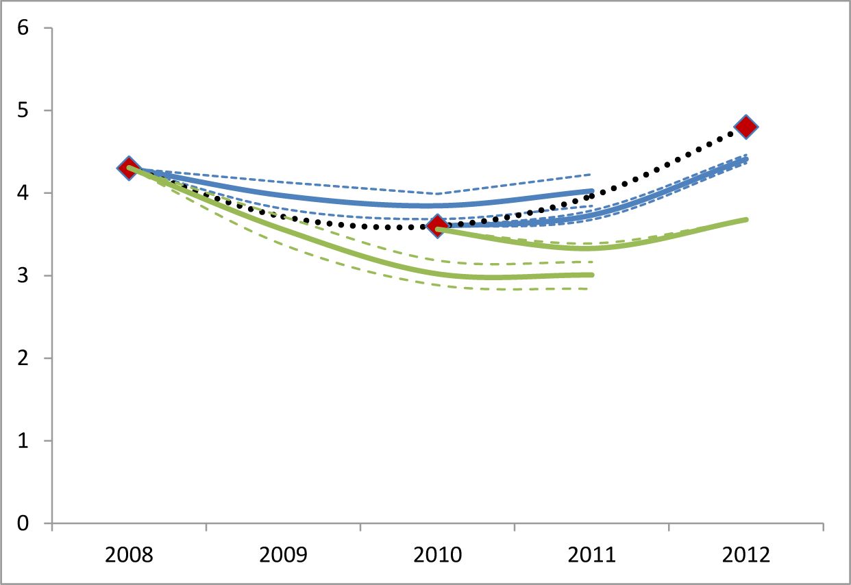
4.1 Backtesting
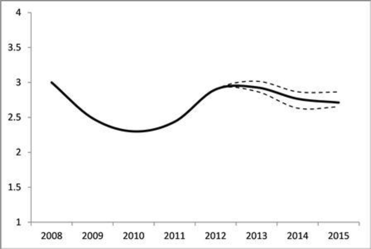
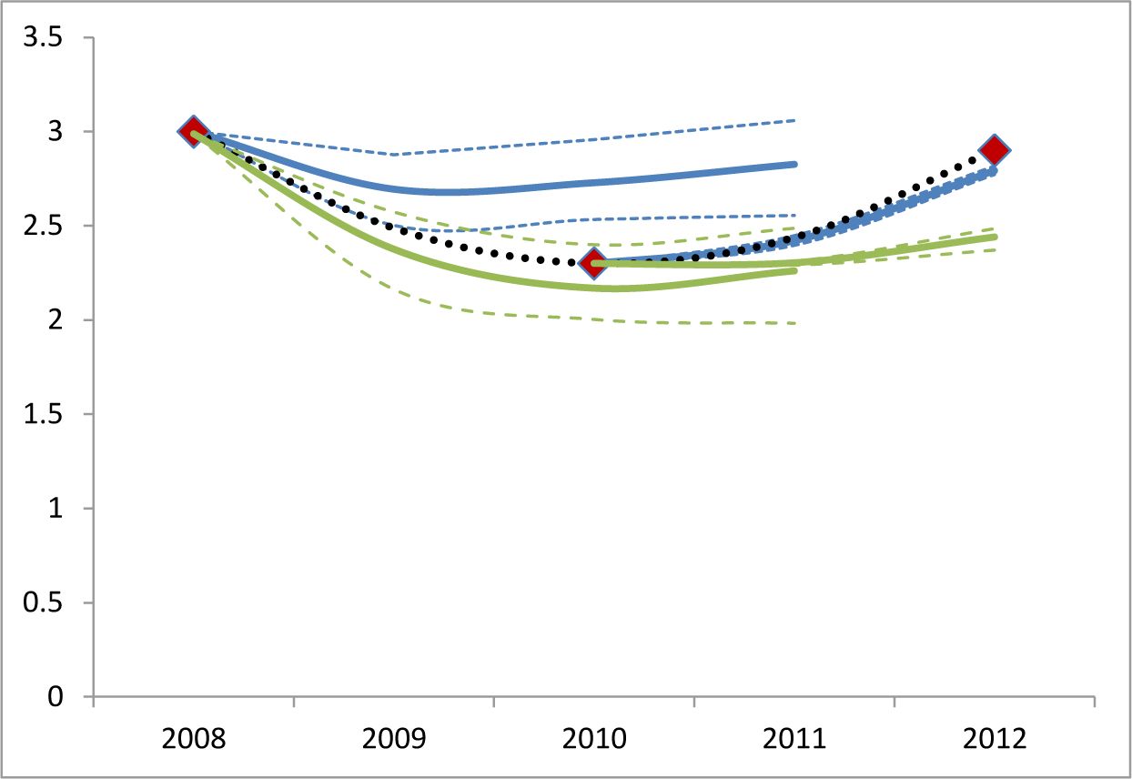
To test the forecasting performance of our model we perform a backtest on previous waves of the SHIW (2008 and 2010). The main results of those simulations are reported in Figure 1 and Figure 2. In particular, we show the percentage of all vulnerable households and of those with income below the median over total households.
In the following figures red diamonds are historical SHIW data. The values for 2009 and 2011 have been interpolated by cubic splines. The solid blue lines are projections of the median value of the share of vulnerable households across 50 simulations, while the dashed lines represent the 10th and 90th percentiles.18
on average, we are able to replicate quite well the percentage of vulnerable households in 2010 and 2012 starting from the 2008 and 2010 waves. The differences between the model results and the data are due to two main factors. First, the SHIW data are an unbalanced panel, in which only half of the sample is maintained in the next wave. As the composition of households can change there could be differences in the total share of vulnerable households and in their characteristics.
Second, there is some measurement error as is common in any household survey.
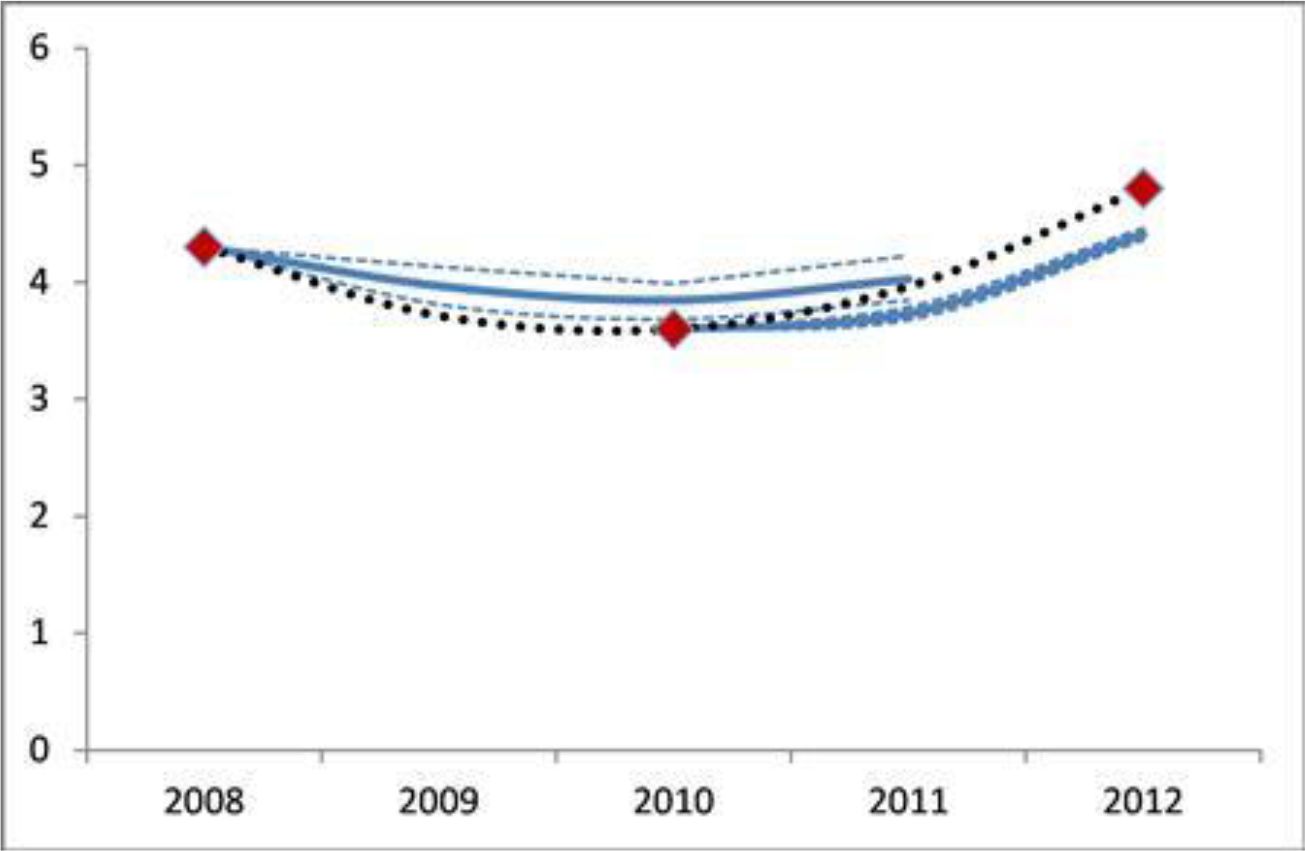

Percentage of vulnerable households in the population.
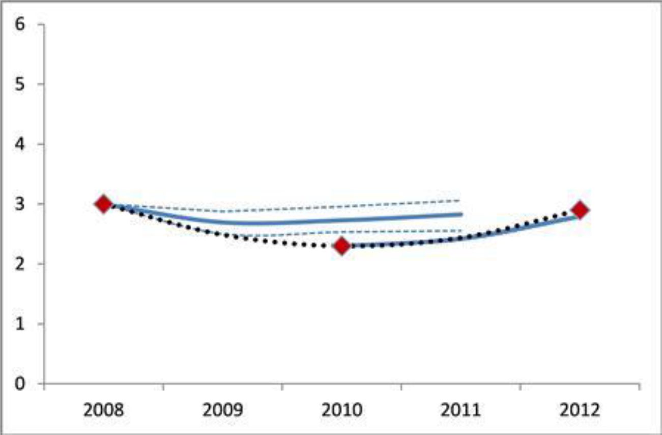
Percentage of vulnerable households with income below the median.
4.2 Baseline scenario
Figure 3 reports the distribution of the debt-service ratio among indebted households in the initial year 2012 and in 2015. The share of indebted households with DSR above 30 per cent is about constant in the two periods.
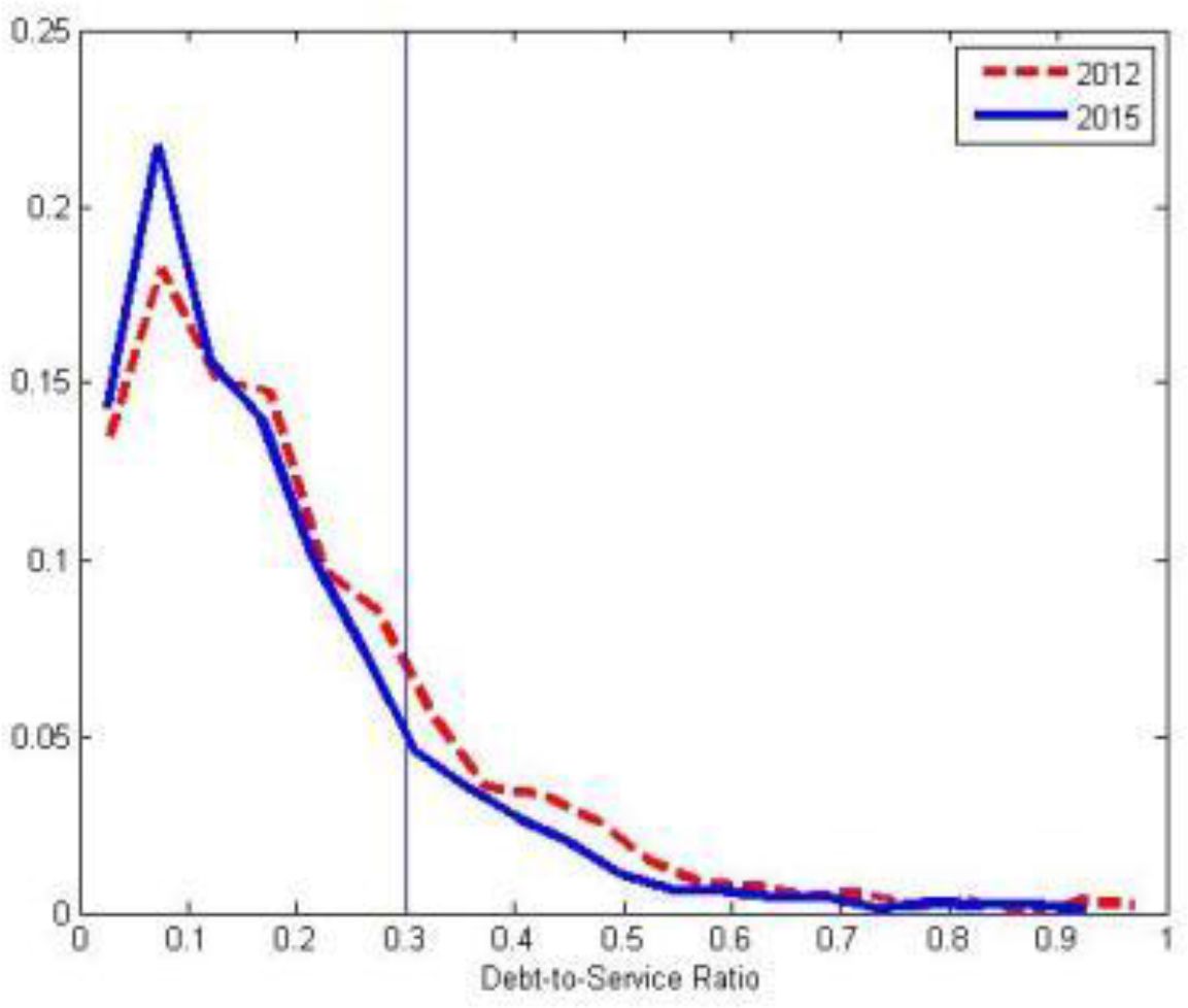
DSR Distribution.
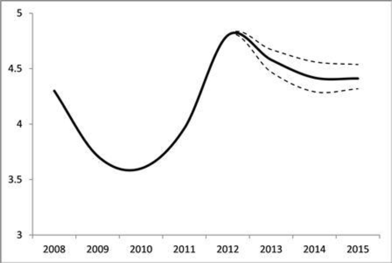
Figure 4 shows the evolution of the fraction of vulnerable households in the total population in the baseline scenario. That share is expected to decrease between 2012 and 2015, moving to about 4.4 per cent. As reported in Table 7, the confidence interval for this value is rather narrow as 80 per cent of the observations are comprised within 4.3 and 4.5 per cent. In 2013, the reduction in the share of vulnerable households is driven by the decrease in the interest rate as households with variable interest rate mortgages pay lower instalments. To a minor extent that reduction is also associated with negative credit growth. In 2014 and in 2015 positive income growth drives the low share of vulnerable households, which decreases slightly relative to 2013. In particular, in 2015 the expected increase in income growth is even larger than in 2014, but at the same time the increase in total debt growth in the economy generates an increase in indebted households, inducing a composition effect. However, in line with the supply conditions observed in recent years, it can be argued that new loans are mostly given to non-vulnerable households19 and, as a result, in 2015 new originations can only explain about 0.4 percentage points of the increase in the share of vulnerable households.20

Percentage of vulnerable households in the population.
In Figure 5, we focus on the percentage of vulnerable households with income below the median. That percentage is about stable between 2012 and 2013 with a slight decrease of 0.2 percentage points in 201521, falling in the range of 2.7–2.9 per cent (see Table 8): the decrease is almost completely driven by positive income growth. Those numbers suggest that also among households with income below the median there are no major risks for financial stability.
Percentage of vulnerable households with income below the median in total households.
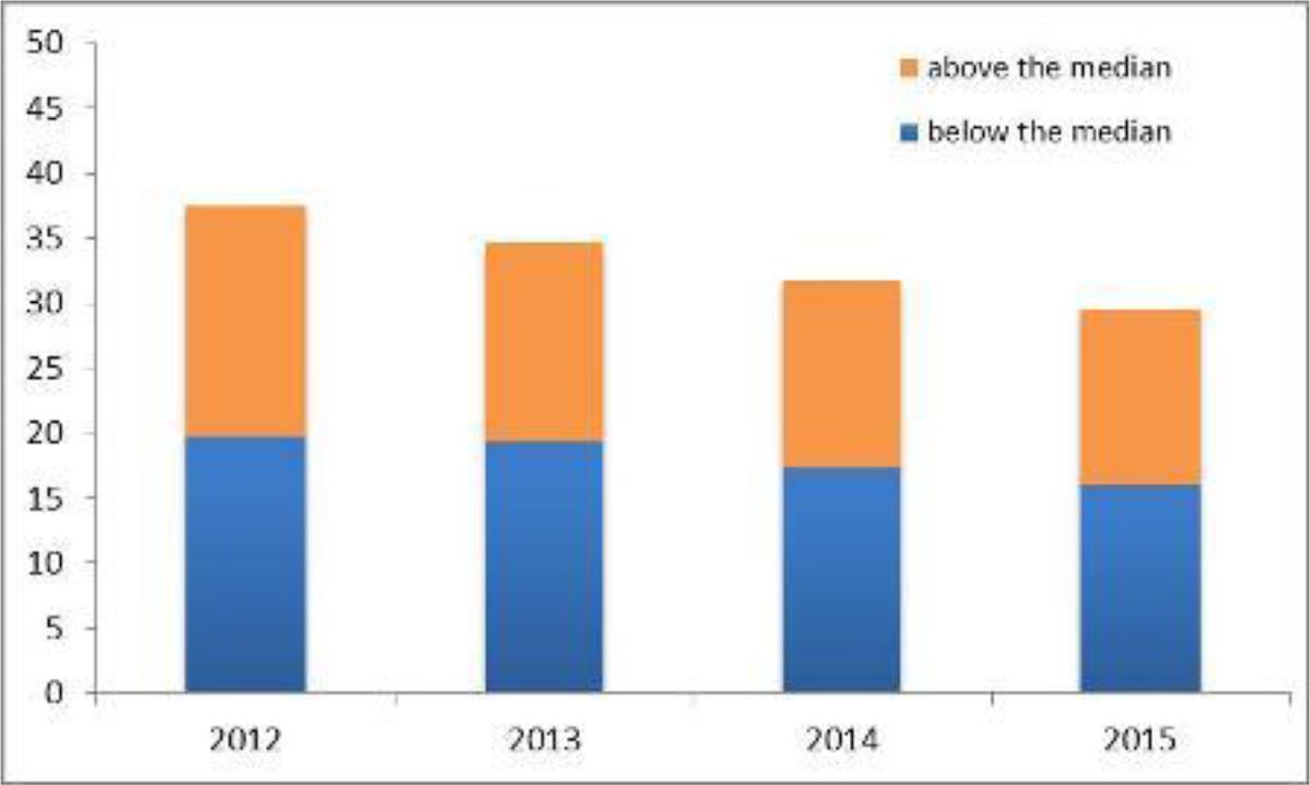
Figure 6 presents the percentage of total debt held by vulnerable households, distinguishing between those belonging to the lower (below the median) and the upper (above the median) groups of equalized income. Those percentages decrease between 2012 and 2015. The share of total debt held by vulnerable households with income below the median moves from 20 per cent to 16 per cent, in line with the estimates for 2010. Similar to 2010, the increase in income growth reduces the percentage of vulnerable households; at the same time, the increase in the total debt growth in 2015 is mainly directed towards households with a low level of vulnerability, so that the share of total debt held by vulnerable households does not increase significantly regardless of a positive growth of total debt in the economy.
Percentage of debt held by all vulnerable households.
Note: above and below the median income.
In Table 6 we report the characteristics of all vulnerable households. Some trends are evident. Vulnerable households belong mainly to the 35-to-54 age group, have secondary education and are in work.
Percentage of vulnerable households by age, education and occupation (Mean values).
| 2012 | 2013 | 2014 | 2015 | Total population (2012) | |
|---|---|---|---|---|---|
| Age | |||||
| < 35 | 16.8 | 14.2 | 12.9 | 10.7 | 9.5 |
| 35–44 | 33.5 | 31.1 | 29.3 | 28.9 | 20.2 |
| 45–54 | 28.4 | 32.7 | 35.0 | 35.7 | 21.3 |
| 55–64 | 9.4 | 9.6 | 11.0 | 12.2 | 16.2 |
| > 65 | 11.9 | 11.9 | 11.3 | 12.1 | 32.8 |
| Education | |||||
| No education or primary education | 6.2 | 6.3 | 6.3 | 6.1 | 23.3 |
| Lower secondary education | 39.7 | 38.4 | 38.3 | 36.0 | 35.8 |
| Upper secondary education | 39.7 | 40.7 | 41.2 | 45.3 | 27.8 |
| Undergraduate or post-graduate | 14.5 | 14.8 | 14.4 | 13.6 | 13.1 |
| Occupation | |||||
| Not working | 16.0 | 15.7 | 15.1 | 14.4 | 41.0 |
| Working | 84.0 | 84.2 | 84.4 | 85.4 | 59.0 |
4.3 Extended baseline scenario and stress test scenarios
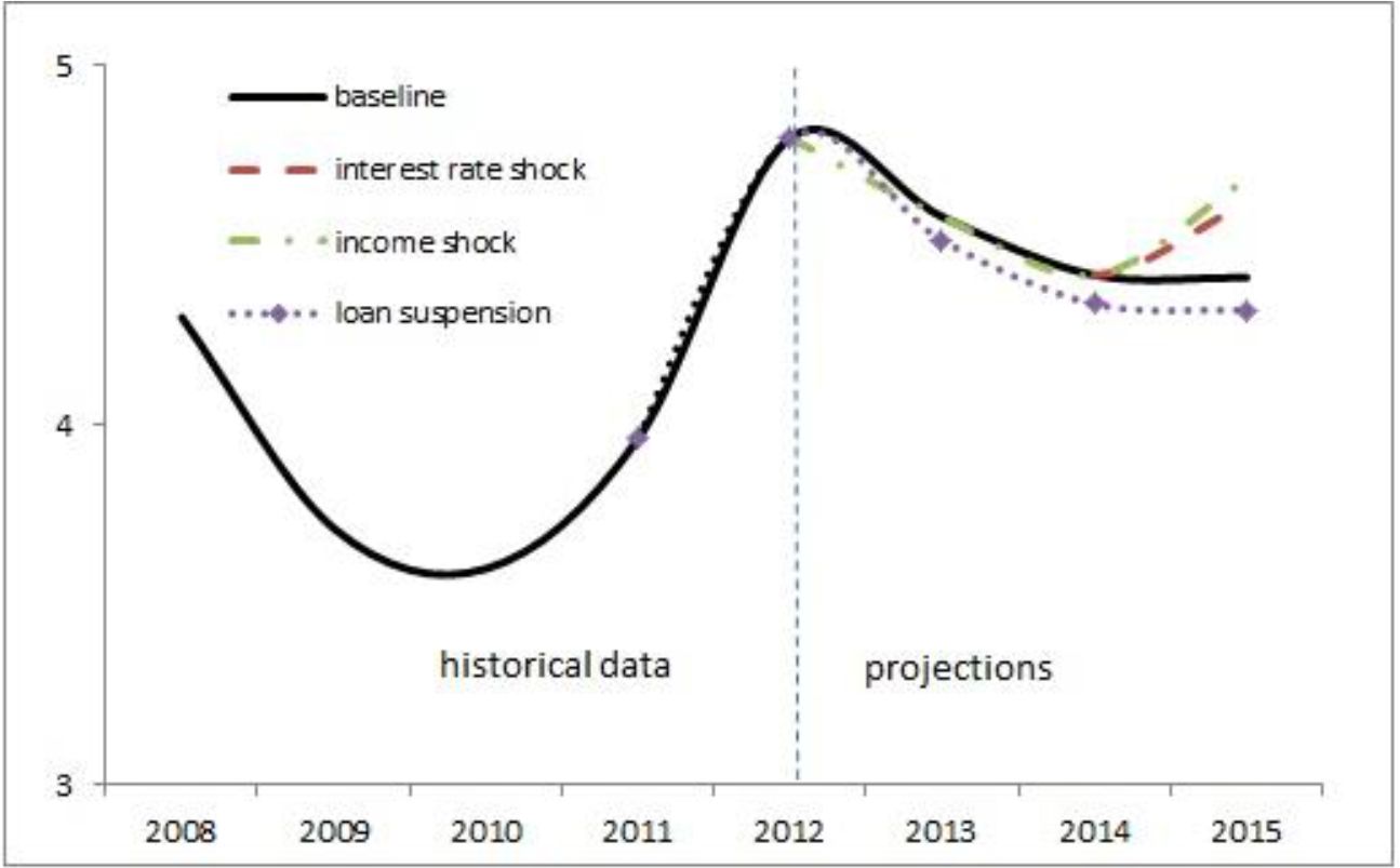
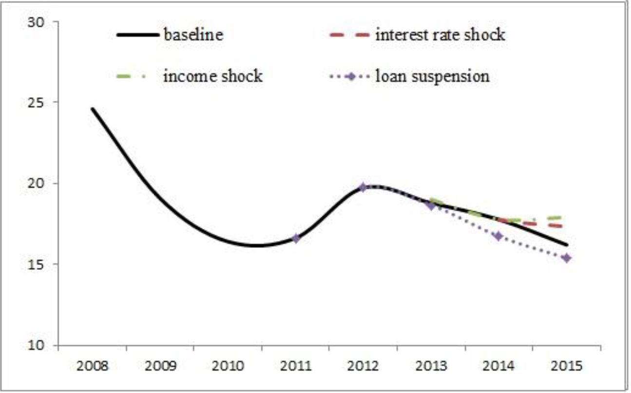
In this section we present an extended baseline scenario and two stress test scenarios. Figure 7 shows how the percentage of all vulnerable households changes in each scenario. Table 7 reports both the median estimates and ranges. Detailed tables with results are reported in the online Appendix.
In the extended baseline scenario we consider the baseline changes in income, interest rate, and total debt (Table 1), but we also include the possibility of obtaining a temporary suspension of mortgage payments for a specific period of time. This option was widely used in the period 2009–12, even with bilateral agreements with banks. The cure rate was quite high: more than 60 per cent of households that obtained suspensions started to repay the mortgage (Bartiloro, Carpinelli, Finaldi Russo & Pastorelli, 2012). We assume that this option is still available until 2015. We modelled it following the data from the 2012 SHIW wave, according to which, between 2009 and 2012, 22 per cent of households with a mortgage belonging to the first income class and 9 per cent of those in the second income class obtained a suspension of mortgage payments over the period. Under this scenario, the percentage of vulnerable households with income below the median drops to 2.6 per cent in 2015, hence it is on average 0.1 percentage points lower than in the baseline scenario. 22
We also consider two alternative scenarios of stress for the financial conditions of indebted households. First, we consider an increase of 100 basis points in the Euribor rate in 2015 (from 0.3% to 1.3%). That increase affects both the loan payments associated with existing variable interest rate mortgages and new mortgage originations.23 Relative to the baseline scenario, the share of all vulnerable households increases by about 0.2 percentage points and their debt increases by about 2 percentage points.
Second, we consider an adverse scenario in which income growth is equal to zero in 2015. The shock affects all households. Relative to the baseline scenario the share of all vulnerable households is about 0.3 percentage points higher and their debt about 2 percentage points higher.
Percentage of vulnerable households under alternative scenarios.
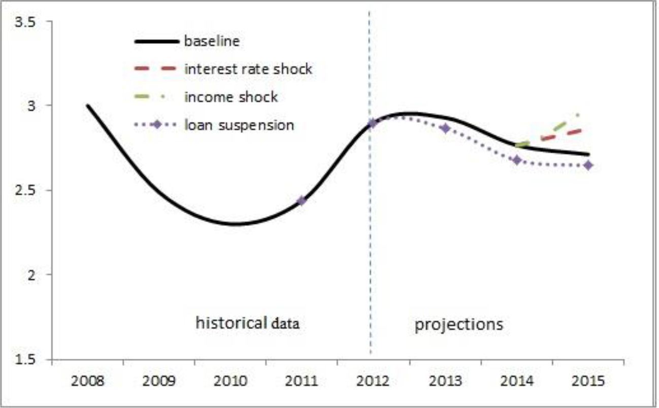
Figure 8 gives the results for vulnerable households belonging to the first two income classes, namely those with income below the median. The mechanisms described above apply and the share of vulnerable households tends to increase slightly following a rise in the Euribor rate or a decrease in nominal income growth.
Percentage of vulnerable households with income below the median under alternative scenarios.
Table 7 and Table 8 report the central estimates and ranges for the baseline case, the extended baseline with suspension of the payments, and the two stress test scenarios that underlie Figure 7 and Figure 8.
Percentage of vulnerable households under alternative scenarios.
| 2012 | 2013 | 2014 | 2015 | ||||
|---|---|---|---|---|---|---|---|
| Baseline | Suspension of payments | Interest rate shock | Income shock | ||||
| Central estimate | 4.8 | 4.6 | 4.4 | 4.4 | 4.3 | 4.6 | 4.7 |
| 10th-90th percentiles | -- | 4.5–4.7 | 4.3–4.6 | 4.3–4.5 | 4.2–4.5 | 4.5–4.7 | 4.6–4.8 |
Percentage of vulnerable households with income below the median under alternative scenarios.
| 2012 | 2013 | 2014 | 2015 | ||||
|---|---|---|---|---|---|---|---|
| Baseline | Suspension of payments | Interest rate shock | Income shock | ||||
| Central estimate | 2.9 | 2.9 | 2.8 | 2.7 | 2.6 | 2.9 | 3.0 |
| 10th-90th percentiles | -- | 2.9–3.0 | 2.6–2.9 | 2.7–2.9 | 2.6–2.8 | 2.7–3.0 | 2.9–3.1 |
Figure 9 shows how the share of total debt held by vulnerable households with income below the median evolves over time in the baseline scenario and in the alternative scenarios described above. In the baseline scenario, the debt held by those vulnerable households tends to decrease from about 20 per cent in 2012 to about 16 per cent in 2015, a level similar to the one recorded in 2010. The reduction is smaller if shocks to income or interest rate occur.

Percentage of total debt held by vulnerable households with income below the median.
4.4 Alternative definition of vulnerability: DSR above 40 per cent
Some central banks and policy institutions (Bank of Canada, FSR 2012; ECB, 2013) define a household as vulnerable if its DSR is equal or above 40 per cent. We implemented the same approach and re-computed the percentage of vulnerable households according to the new, less stringent definition. As shown in Figure 10 the share of vulnerable households now equals 2.3 per cent in 2012 and it is projected to decrease slightly over time, to 2.1 per cent in 2015. As mentioned before, the reduction is mostly driven by the positive income growth.
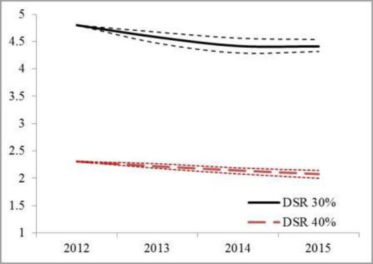
Percentage of vulnerable households with DSR above 40%.
5. Conclusions
This paper presents a framework to study how the vulnerability of Italian households evolves over time. Starting from the SHIW microeconomic data and incorporating some macroeconomic projections on income growth, total debt growth and interest rates, we built a model that captures the evolution of households’ debt and vulnerability over time. The micro-founded model delivers aggregate variables that are in line with projected macroeconomic statistics and is therefore suitable for simulating stress scenarios to evaluate households’ resilience to negative shocks, such as income or interest rate shocks. The model is also well suited to study the effects of stress scenarios, alternative policy measures or the effects associated with the suspension of loan payments driven by banks’ decisions.
We found that the percentage of vulnerable households with equalized income below the median is projected to be almost stable between 2012 and 2015, being in the order of 2.7 per cent in 2015. Similarly, the share of total debt held by those vulnerable households decreases progressively to 16 per cent in 2015, a value similar to the one in 2010. When simulating scenarios of stress, zero income growth has a larger effect on the share of vulnerable households than a 100 basis point increase in interest rates.
Future research aims to improve the current model. First of all, we could include a probability of becoming unemployed. Households facing spells of unemployment of different severity and duration may become vulnerable and so could raise the percentage of vulnerable households. Other important factors of vulnerability which can be simulated starting from our microdata could be incorporated. For instance, changes in household composition due to birth of a child or divorce may affect the income committed to debt repayment and thus the ability to service the debt. Second, we could try to incorporate other sources of macroeconomic data when modelling new mortgage originations. Third, we could study other indicators of households’ vulnerability and accordingly evaluate their evolution over time. Fourth, we could improve our modelling approach for consumer credit debt.
Finally, one related question that could be addressed in some future work is whether the dynamics of the mortgage debt has any impact on the outcome indicators at the micro-level. In particular, it would be worth analysing how the mortgage debt affects some groups of households that are especially prone to the risk of unemployment and poverty in Italy, e.g. young people households.
Footnotes
1.
It currently stands at around 63 per cent of disposable income. See Bank of Italy (2014).
2.
This is particularly true for the highest income groups. A back test exercise keeping the share of principal on current balance fixed is reported in the online Appendix.
3.
This result follows, to a minor extent, from our assumption that lending standards will remain somewhat tight in the next few years compared with the levels observed before the financial crisis.
4.
For a general description of the survey, see http://www.bancaditalia.it/statistiche/tematiche/indagini-famiglie-imprese/bilanci-famiglie/index.html?com.dotmarketing.htmlpage.language=1
5.
The data allow us to differentiate between first mortgage, second mortgage and third mortgage on the primary residence and on other real estate.
6.
Studies based on data provided by financial intermediaries indicate a higher fraction of households with variable rate mortgages (see Felici et al., 2012). We also tested our model assuming 70 per cent of mortgages with variable rate (see the online Appendix); the results are overall confirmed.
7.
As explained below, in the computation of the DSR we use the disposable income gross of financial charges and net of imputed rent, which better captures the monetary income available to the household for consumption or as a buffer against unexpected shocks. In the model we keep track of both definitions of income to be able both to match the macroeconomic aggregates and to compute correctly the DSR. The equalized income, computed starting from the disposable income and using the OECD equivalence scale, is used to group households into four income classes.
8.
The model has been used to evaluate the evolution of households’ vulnerability in accordance with the economic slowdown registered as November 2014. We used a baseline scenario in which both nominal income and lending to households begin to rise again only in 2015 and interest rates remain almost unchanged. For an overview of the simulation results see Financial Stability Report No. 2, November 2014, Bank of Italy.
9.
Those projections on total debt growth were developed in April 2014.
10.
Euribor is short for Euro Interbank Offered Rate. It is defined as “the rate at which Euro interbank term deposits are offered by one prime bank to another prime bank within the EMU zone” (http://www.emmi-benchmarks.eu/euribor-org/about-euribor.html).
11.
An alternative assumption for new originations, relying on projections of interest rates on loans for house purchase developed at Bank of Italy, has been tested. The results of the simulation exercise (available upon request) do not differ significantly from the ones presented here.
12.
Data on the Euribor rate refer to March in each year.
13.
The value of imputed rents is provided by each household in the survey. The related questions are: “Imagine you wanted to let your house/flat, what monthly rent do you or the household think could be charged? Do not include condominium charges, heating or other expenses.” and “If you wanted to let the property, what annual rental could the household obtain? total amount in the year.”
14.
Alternatively, to estimate the mean and standard deviation of the income process we could have used the SHIW data from 2008 to 2012. This sample captures the slowdown of the Italian economy and therefore would be adequate if the recession were to continue. As shown in the online Appendix, the estimated income means associated with the period 2008–12 are negative, but the mean growth is less negative for the 75st-100th percentile and more negative for the 1st-25th percentile, indicating that households in the lowest group are those that suffer the most. In periods of expansion and in periods of recession income movements for the lowest income group are stronger and therefore it is important to take them properly into account. We also present a sensitivity test using as income parameters those estimated using the 2008–12 sample period and we find that the share of vulnerable households is projected to be slightly higher than in the baseline scenario.
15.
The share of households renegotiating a mortgage contract was about 2 per cent in 2012, while the share of those refinancing it was below 3 per cent (Source: Regional Lending Banking Survey).
16.
See e.g. Financial Stability Report No. 6, November 2013, Bank of Italy.
17.
In the code we set θk,t=0.5·θk,t-2 the first period as the survey is biannual.
18.
A further backtesting exercise is reported in the online Appendix. In that exercise we also present the results for the assumption of an amortization schedule in which the share of principal on current credit balance is kept fixed, as in Djoudad (2010).
19.
This result is confirmed by the case with no originations reported in the online Appendix, where the dynamics for the share of vulnerable households in the population is very similar to the case with originations. This result suggests that changes in interest rates or in income are the primary driving forces of households’ vulnerability.
20.
This result is obtained comparing the baseline scenario with the scenario without originations.
21.
This result is based on a comparison of the median values obtained across simulations in different years.
22.
This result and the following comparisons with the baseline scenario are based on the difference between median values obtained across simulations under alternative economic scenarios.
23.
We assume that the interest rate change has no effect on consumer debt.
Online appendix
1. Detailed results
1.1 Baseline scenario
| 2012 | 2013 | 2014 | 2015 | |
|---|---|---|---|---|
| Percentage of vulnerable households over total households | ||||
| 1st–25th percentile | 1.5 | 1.6 | 1.6 | 1.6 |
| 25th–50th percentile | 1.4 | 1.4 | 1.2 | 1.1 |
| Below the median | 2.9 | 2.9 | 2.8 | 2.7 |
| 50th–75th percentile | 1.2 | 1.0 | 0.9 | 0.8 |
| 75th–100th percentile | 0.7 | 0.7 | 0.7 | 0.8 |
| TOTAL | 4.8 | 4.6 | 4.4 | 4.4 |
| Percentage of vulnerable households over indebted households | ||||
| 1st–25th percentile | 7.6 | 7.4 | 6.8 | 6.7 |
| 25th–50th percentile | 7.0 | 6.3 | 5.2 | 4.6 |
| Below the median | 14.6 | 13.6 | 12.0 | 11.2 |
| 50th–75th percentile | 6.0 | 4.4 | 3.8 | 3.3 |
| 75th–100th percentile | 3.5 | 3.0 | 3.2 | 3.3 |
| TOTAL | 24.1 | 21.2 | 19.1 | 18.1 |
| Percentage of debt held by vulnerable households | ||||
| 1st–25th percentile | 9.5 | 10.4 | 9.7 | 9.2 |
| 25th–50th percentile | 10.2 | 9.1 | 7.9 | 7.0 |
| Below the median | 19.7 | 19.3 | 17.4 | 16.0 |
| 50th–75th percentile | 7.9 | 6.4 | 5.9 | 5.2 |
| 75th–100th percentile | 9.8 | 9.1 | 8.7 | 8.2 |
| TOTAL | 37.5 | 34.7 | 31.8 | 29.5 |
-
Note: Households are divided into classes according to their equalized income gross of imputed rents. The reported values have been approximated to the first decimal.
1.2 Suspension of loan payments

| 2012 | 2013 | 2014 | 2015 | |
|---|---|---|---|---|
| Percentage of vulnerable households over total households | ||||
| 1st–25th percentile | 1.5 | 1.6 | 1.5 | 1.6 |
| 25th–50th percentile | 1.4 | 1.3 | 1.2 | 1.1 |
| Below the median | 2.9 | 2.9 | 2.7 | 2.6 |
| 50th–75th percentile | 1.2 | 1.0 | 0.9 | 0.8 |
| 75th–100th percentile | 0.7 | 0.7 | 0.7 | 0.8 |
| TOTAL | 4.8 | 4.5 | 4.3 | 4.3 |
| Percentage of vulnerable households over indebted households | ||||
| 1st–25th percentile | 7.6 | 7.2 | 6.5 | 6.4 |
| 25th–50th percentile | 7.0 | 6.2 | 5.2 | 4.4 |
| Below the median | 14.6 | 13.3 | 11.6 | 10.9 |
| 50th–75th percentile | 6.0 | 4.4 | 3.8 | 3.3 |
| 75th–100th percentile | 3.5 | 3.0 | 3.2 | 3.3 |
| TOTAL | 24.1 | 20.9 | 18.8 | 17.8 |
| Percentage of debt held by vulnerable households | ||||
| 1st–25th percentile | 9.5 | 10.1 | 9.1 | 8.8 |
| 25th–50th percentile | 10.2 | 8.9 | 7.9 | 6.8 |
| Below the median | 19.7 | 18.7 | 16.7 | 15.4 |
| 50th–75th percentile | 7.9 | 6.4 | 5.9 | 5.2 |
| 75th–100th percentile | 9.8 | 9.1 | 8.7 | 8.2 |
| TOTAL | 37.5 | 34.0 | 31.4 | 29.1 |
1.3 Stress test scenarios
1.3.1 Interest rate shock

| 2012 | 2013 | 2014 | 2015 | |
|---|---|---|---|---|
| Percentage of vulnerable households over total households | ||||
| 1st–25th percentile | 1.5 | 1.6 | 1.6 | 1.7 |
| 25th–50th percentile | 1.4 | 1.4 | 1.2 | 1.2 |
| Below the median | 2.9 | 2.9 | 2.8 | 2.9 |
| 50th–75th percentile | 1.2 | 1.0 | 0.9 | 0.9 |
| 75th–100th percentile | 0.7 | 0.7 | 0.7 | 0.8 |
| TOTAL | 4.8 | 4.6 | 4.4 | 4.6 |
| Percentage of vulnerable households over indebted households | ||||
| 1st–25th percentile | 7.6 | 7.4 | 6.8 | 6.9 |
| 25th–50th percentile | 7.0 | 6.3 | 5.2 | 4.9 |
| Below the median | 14.6 | 13.6 | 12.0 | 11.8 |
| 50th–75th percentile | 6.0 | 4.4 | 3.8 | 3.5 |
| 75th–100th percentile | 3.5 | 3.0 | 3.2 | 3.4 |
| TOTAL | 24.1 | 21.2 | 19.1 | 19.0 |
| Percentage of debt held by vulnerable households | ||||
| 1st–25th percentile | 9.5 | 10.4 | 9.7 | 9.7 |
| 25th–50th percentile | 10.2 | 9.1 | 7.9 | 7.6 |
| Below the median | 19.7 | 19.3 | 17.4 | 17.1 |
| 50th–75th percentile | 7.9 | 6.4 | 5.9 | 5.7 |
| 75th–100th percentile | 9.8 | 9.1 | 8.7 | 8.7 |
| TOTAL | 37.5 | 34.7 | 31.8 | 31.4 |
1.3.2 Income shock

| 2012 | 2013 | 2014 | 2015 | |
|---|---|---|---|---|
| Percentage of vulnerable households over total households | ||||
| 1st–25th percentile | 1.5 | 1.6 | 1.6 | 1.7 |
| 25th–50th percentile | 1.4 | 1.4 | 1.2 | 1.3 |
| Below the median | 2.9 | 2.9 | 2.8 | 3.0 |
| 50th–75th percentile | 1.2 | 1.0 | 0.9 | 0.9 |
| 75th–100th percentile | 0.7 | 0.7 | 0.7 | 0.7 |
| TOTAL | 4.8 | 4.6 | 4.4 | 4.7 |
| Percentage of vulnerable households over indebted households | ||||
| 1st–25th percentile | 7.6 | 7.4 | 6.8 | 6.9 |
| 25th–50th percentile | 7.0 | 6.3 | 5.2 | 5.4 |
| Below the median | 14.6 | 13.6 | 12.0 | 12.3 |
| 50th–75th percentile | 4.0 | 4.4 | 3.8 | 3.8 |
| 75th–100th percentile | 3.5 | 3.0 | 3.2 | 3.0 |
| TOTAL | 24.1 | 21.2 | 19.1 | 19.3 |
| Percentage of debt held by vulnerable households | ||||
| 1st–25th percentile | 9.5 | 10.4 | 9.7 | 9.5 |
| 25th–50th percentile | 10.2 | 9.1 | 7.9 | 8.0 |
| Below the median | 19.7 | 19.3 | 17.4 | 17.3 |
| 50th–75th percentile | 7.9 | 6.4 | 5.9 | 5.5 |
| 75th–100th percentile | 9.8 | 9.1 | 8.7 | 8.2 |
| TOTAL | 37.5 | 34.7 | 31.8 | 31.2 |
1.4 Households are vulnerable if DSR > 40%

| 2012 | 2013 | 2014 | 2015 | |
|---|---|---|---|---|
| Percentage of vulnerable households over total households | ||||
| 1st–25th percentile | 1.0 | 1.0 | 1.0 | 1.0 |
| 25th–50th percentile | 0.6 | 0.6 | 0.5 | 0.5 |
| Below the median | 1.6 | 1.6 | 1.5 | 1.4 |
| 50th–75th percentile | 0.4 | 0.3 | 0.3 | 0.3 |
| 75th–100th percentile | 0.3 | 0.3 | 0.3 | 0.3 |
| TOTAL | 2.3 | 2.2 | 2.1 | 2.1 |
| Percentage of vulnerable households over indebted households | ||||
| 1st–25th percentile | 4.8 | 4.5 | 4.2 | 4.1 |
| 25th–50th percentile | 3.1 | 2.7 | 2.2 | 1.9 |
| Below the median | 7.9 | 7.3 | 6.4 | 5.9 |
| 50th–75th percentile | 2.1 | 1.6 | 1.3 | 1.2 |
| 75th–100th percentile | 1.5 | 1.3 | 1.3 | 1.3 |
| TOTAL | 11.5 | 10.2 | 9.2 | 8.5 |
| Percentage of debt held by vulnerable households | ||||
| 1st–25th percentile | 6.6 | 6.9 | 6.3 | 5.8 |
| 25th–50th percentile | 4.9 | 4.2 | 3.6 | 3.0 |
| Below the median | 11.5 | 11.1 | 9.9 | 8.6 |
| 50th–75th percentile | 3.4 | 3.0 | 2.5 | 2.1 |
| 75th–100th percentile | 3.3 | 3.1 | 3.1 | 2.9 |
| TOTAL | 18.2 | 17.1 | 15.7 | 13.8 |
1.5 No originations

| 2012 | 2013 | 2014 | 2015 | ||
|---|---|---|---|---|---|
| Percentage of vulnerable households over total households | |||||
| 1st–25th percentile | 1.5 | 1.6 | 1.4 | 1.3 | |
| 25th–50th percentile | 1.4 | 1.4 | 1.2 | 1.0 | |
| Below the median | 2.9 | 2.9 | 2.6 | 2.3 | |
| 50th–75th percentile | 1.2 | 1.0 | 0.9 | 0.8 | |
| 75th–100th percentile | 0.7 | 0.7 | 0.7 | 0.8 | |
| TOTAL | 4.8 | 4.6 | 4.3 | 4.0 | |
| Percentage of vulnerable households over indebted households | |||||
| 1st–25th percentile | 7.6 | 8.0 | 7.5 | 7.0 | |
| 25th–50th percentile | 7.0 | 6.9 | 6.1 | 5.1 | |
| Below the median | 14.6 | 14.7 | 13.5 | 12.1 | |
| 50th–75th percentile | 6.0 | 4.8 | 4.5 | 4.2 | |
| 75th–100th percentile | 3.5 | 3.3 | 3.7 | 4.1 | |
| TOTAL | 24.1 | 23.0 | 21.9 | 20.8 | |
| Percentage of debt held by vulnerable households | |||||
| 1st–25th percentile | 9.5 | 10.7 | 10.1 | 9.7 | |
| 25th–50th percentile | 10.2 | 9.4 | 8.6 | 7.4 | |
| Below the median | 19.7 | 19.9 | 18.3 | 16.9 | |
| 50th–75th percentile | 7.9 | 6.7 | 6.5 | 6.1 | |
| 75th–100th percentile | 9.8 | 9.4 | 9.6 | 9.7 | |
| TOTAL | 37.5 | 35.9 | 34.1 | 32.8 | |
1.6 Credit loans and 70 % of mortgages at adjustable rate

| 2012 | 2013 | 2014 | 2015 | |
|---|---|---|---|---|
| Percentage of vulnerable households over total households | ||||
| 1st–25th percentile | 1.5 | 1.6 | 1.6 | 1.6 |
| 25th–50th percentile | 1.4 | 1.3 | 1.2 | 1.1 |
| Below the median | 2.9 | 2.9 | 2.7 | 2.7 |
| 50th–75th percentile | 1.2 | 0.9 | 0.9 | 0.8 |
| 75th–100th percentile | 0.7 | 0.7 | 0.7 | 0.8 |
| TOTAL | 4.8 | 4.5 | 4.4 | 4.4 |
| Percentage of vulnerable households over indebted households | ||||
| 1st–25th percentile | 7.6 | 7.4 | 6.8 | 6.6 |
| 25th–50th percentile | 7.0 | 6.2 | 5.1 | 4.5 |
| Below the median | 14.6 | 13.4 | 11.9 | 11.2 |
| 50th–75th percentile | 6.0 | 4.2 | 3.8 | 3.3 |
| 75th–100th percentile | 3.5 | 3.0 | 3.1 | 3.3 |
| TOTAL | 24.1 | 20.8 | 18.9 | 18.0 |
| Percentage of debt held by vulnerable households | ||||
| 1st–25th percentile | 9.5 | 10.4 | 9.6 | 9.2 |
| 25th–50th percentile | 10.2 | 8.9 | 7.8 | 6.9 |
| Below the median | 19.7 | 18.9 | 17.2 | 15.9 |
| 50th–75th percentile | 7.9 | 6.3 | 5.8 | 5.2 |
| 75th–100th percentile | 9.8 | 8.9 | 8.6 | 8.2 |
| TOTAL | 37.5 | 34.2 | 31.3 | 29.3 |
-
Note: we randomly assigned a fraction of individuals declaring a fixed rate mortgage to hold a variable rate mortgage so that about 70 per cent of the mortgages are at variable rate. We also assume that the credit loans are adjustable rate.
1.7 Income process estimated using the SHIW data from 2008 to 2012
Estimated mean and standard deviation for the income process (SHIW 2008-2012).
| yd growth | y growth | |||
|---|---|---|---|---|
| μd | σd | μ | σ | |
| 1st – 25th percentile | -0.020 | 0.040 | -0.028 | 0.032 |
| 25th – 50th percentile | -0.014 | 0.029 | -0.016 | 0.025 |
| 50th – 75th percentile | -0.014 | 0.036 | -0.014 | 0.025 |
| 75th – 100th percentile | -0.010 | 0.029 | -0.011 | 0.001 |
| 2012 | 2013 | 2014 | 2015 | |
|---|---|---|---|---|
| Percentage of vulnerable households over total households | ||||
| 1st–25th percentile | 1.5 | 1.6 | 1.7 | 1.8 |
| 25th–50th percentile | 1.4 | 1.4 | 1.3 | 1.2 |
| Below the median | 2.9 | 3.0 | 3.0 | 3.0 |
| 50th–75th percentile | 1.2 | 0.9 | 0.9 | 0.8 |
| 75th–100th percentile | 0.7 | 0.7 | 0.7 | 0.7 |
| TOTAL | 4.8 | 4.6 | 4.5 | 4.6 |
| Percentage of vulnerable households over indebted households | ||||
| 1st–25th percentile | 7.6 | 7.5 | 7.3 | 7.3 |
| 25th–50th percentile | 7.0 | 6.4 | 5.5 | 4.9 |
| Below the median | 14.6 | 13.9 | 12.8 | 12.4 |
| 50th–75th percentile | 6.0 | 4.4 | 3.8 | 3.4 |
| 75th–100th percentile | 3.5 | 3.0 | 2.9 | 3.0 |
| TOTAL | 24.1 | 21.4 | 19.6 | 18.9 |
| Percentage of debt held by vulnerable households | ||||
| 1st–25th percentile | 9.5 | 10.5 | 10.0 | 9.8 |
| 25th–50th percentile | 10.2 | 9.3 | 8.5 | 7.5 |
| Below the median | 19.7 | 19.7 | 18.4 | 17.1 |
| 50th–75th percentile | 7.9 | 6.2 | 5.7 | 5.1 |
| 75th–100th percentile | 9.8 | 9.1 | 7.8 | 7.8 |
| TOTAL | 37.5 | 35.0 | 32.0 | 30.2 |
-
Note: we randomly assigned a fraction of individuals declaring a fixed rate mortgage to hold a variable rate mortgage so that about 70 percent of the mortgages are at variable rate. We also assume that the credit loans are adjustable rate.
2. Comparison of backtesting exercices under different amortization hypotheses
Percentage of vulnerable households over total population.

Percentage of vulnerable households with income below the median over total population.
Note: The blue lines represent projections assuming a French amortization schedule; the green lines are projections assuming a fixed share of principal on current credit balance.
References
-
1
Financial fragility of euro area households. Working Paper Series 1737 ECBFinancial fragility of euro area households. Working Paper Series 1737 ECB.
- 2
- 3
- 4
-
5
L’accesso al credito in tempo di crisi: le misure di sostegno a imprese e famiglie. Bank of Italy Occasional Papers (Questioni di economia e finanza)111, L’accesso al credito in tempo di crisi: le misure di sostegno a imprese e famiglie. Bank of Italy Occasional Papers (Questioni di economia e finanza).
-
6
The Bank of Canada’s analytic framework for assessing the vulnerability of the household sectorFinancial System Review pp. 57–62.
-
7
The Eurosystem Household, Finance and Consumption Survey, Results from the first wave. Statistics Paper Series 2The Eurosystem Household, Finance and Consumption Survey, Results from the first wave. Statistics Paper Series 2.
-
8
Crisis and Italian Households: A Microeconomic Analysis of Mortgage Contracts. Bank of Italy Occasional Papers (Questioni di economia e finance)125, Crisis and Italian Households: A Microeconomic Analysis of Mortgage Contracts. Bank of Italy Occasional Papers (Questioni di economia e finance).
-
9
Income Risk, Borrowing Constraints, and Portfolio ChoiceAmerican Economic Review, American Economic Association 86:158–72.
-
10
United Kingdom: Vulnerabilities of household and corporate balance sheets and risks for the financial sector Technical Note. Country Report 11/229United Kingdom: Vulnerabilities of household and corporate balance sheets and risks for the financial sector Technical Note. Country Report 11/229.
-
11
Spain: Vulnerabilities of private sector balance sheets and risks to the financial sector Technical Note. Country Report 12/140Spain: Vulnerabilities of private sector balance sheets and risks to the financial sector Technical Note. Country Report 12/140.
-
12
Italy: Technical Note on the financial situation of Italian households and non-financial corporations and risks to the banking system. Country Report No. 13/348Italy: Technical Note on the financial situation of Italian households and non-financial corporations and risks to the banking system. Country Report No. 13/348.
-
13
The dynamics of household wealth accumulation in ItalyFiscal Studies, Institute for Fiscal Studies 21:269–295.
-
14
Does consumption inequality track income inequality in Italy?Review of Economic Dynamics, Elsevier for the Society for Economic Dynamics 13:133–153.
-
15
Italian households’ debt: the participation to the debt market and the size of the loanEmpirical Economics 33:401–426.
-
16
L’indebitamento delle famiglie italiane dopo la crisi del 2008. Bank of Italy Occasional Papers (Questioni di economia e finanza)134, L’indebitamento delle famiglie italiane dopo la crisi del 2008. Bank of Italy Occasional Papers (Questioni di economia e finanza).
-
17
Il mercato del credito alle famiglie dopo cinque anni di crisi: evidenze dall’indagine sui loro bilanci. Bank of Italy Occasional Papers (Questioni di economia e finanza)241, Il mercato del credito alle famiglie dopo cinque anni di crisi: evidenze dall’indagine sui loro bilanci. Bank of Italy Occasional Papers (Questioni di economia e finanza).
-
18
OECD Factjournal 2010: Economic, Environmental and Social Statistics, Paris, OECD PublishingOECD Factjournal 2010: Economic, Environmental and Social Statistics, Paris, OECD Publishing.
Article and author information
Author details
Acknowledgements
Financial Stability Directorate, Bank of Italy. We thank Paolo Angelini, Antonio Di Cesare, Giorgio Gobbi, Silvia Magri, Matteo Piazza, Luigi Federico Signorini the editor and two anonymous referees for their useful comments. The analysis and conclusions expressed herein are those of the authors and should not be attributed to the Bank of Italy.
Publication history
- Version of Record published: December 31, 2014 (version 1)
Copyright
© 2014, Michelangeli & Pietrunti
This article is distributed under the terms of the Creative Commons Attribution License, which permits unrestricted use and redistribution provided that the original author and source are credited.