The quantitative and qualitative evaluation of a multi-agent microsimulation model for subway carriage design
- Tsinghua University, China
- The University of Melbourne, Australia
- Shanghai University of Finance and Economics, China
- Lab MAS, France
Abstract
Multi-agent microsimulation, as a third way of doing science other than induction and deduction methods, is explored to aid subway carriage design in this paper. Realizing that passenger behavior shapes the environment and in turn is shaped by the environment itself, we intend to model this interaction and examine the effectiveness and usability of the proposed model. We address our micro-model from essential aspects of environment space, agent attributes, agent behaviors, simulation process, and global objective/convergence function. Based on the real and simulated data, we evaluate our model with a combination of quantitative and qualitative procedures. For quantitative approach, we proposed two evaluation paradigms (i.e. “unified multinomial classifier” and “one-vs.-all binary classifiers”) using the state-of-the-art machine learning techniques and frameworks; and we manage to show from various perspectives that our model matches the reality in the majority of cases. For qualitative verification, we present a small-scale case study to evaluate different seat layouts in a subway carriage, and identify their advantages and disadvantages with little effort. By enriching microsimulation theory with innovative techniques, our research aims at promoting its acceptance level in design communities by means of avoiding costly creation of real-world experiments.
1. Introduction
The traditional subway carriage design activities can be classified into two categories: induction and deduction approaches. Induction approach includes activities such as requirement analysis and evaluation approaches based on comprehensive user studies, while deduction approach often refers to the design activities that are directed by design principles and designers’ experience. Although both approaches have been applied widely in the domain of subway carriage design, designers are aware of their limitations. Induction approach is weakened by the fact that data from time-consuming user studies are incomplete and biased in most cases. At the mention of the weakness of deduction approach, designers commonly admit that it is difficult to adapt principles and experiences from one specific design field to another, because most design principles only hold within specific social and cultural constrains. Belonging to neither induction nor deduction methodologies, multi-agent microsimulation as an exciting new approach to model the crowd behavior offers us a unique perspective for understanding passenger flow patterns in subway carriages.
As a mandatory effort before applying any micro-model in design activities, the micro-model needs to be evaluated with either qualitative or quantitative approaches. The qualitative study is concerned with complete and detailed descriptions of observations, whereas quantitative evaluation creates statistical models to explain observations; both approaches have several advantages and disadvantages, depending upon the aim and focus of researchers (Goertz & Mahoney, 2012). There is a strong tendency to locate qualitative and quantitative methods in two different methodological paradigms. However, a few frontier researchers have attempted to develop a basis in both technical methods and methodologies for integrating the two approaches. The parallel use of qualitative and quantitative procedures may: converge (tend to agree), constitute a complementary relationship (reciprocally supplement each other), and diverge (contradict each other), (Jenner, Flick, von Kardoff, & Steinke, 2004) which we believe might give an appropriate integral picture for the simulation quality of micro-models.
After briefly reviewing the relevant research areas in Section 1.1 and clarifying our research problems and goals in Section 1.2, we will exhaustively present in Section 2 our multi-agent micro-model from five perspectives: environment space (Section 2.1), agent attributes (Section 2.2), agent behaviors (Section 2.3), simulation process, and global objective function (Section 2.4). As the foundation of model evaluation, we introduce the simulated (via model execution) and real (via in-field observation) data collection in Section 3.1 and 3.2 respectively. Concerning machine learning based quantitative evaluation, we consecutively elaborate on topics of supervised training (Section 3.3.1), multinomial classifier prediction (Section 3.3.2), and one-vs.-all binary classifiers (Section 3.3.3). Finally in Section 3.4, we exemplify a qualitative case study on evaluating different interior seat arrangements in a subway carriage; and conclusions are drawn in Section 4.
1.1 Description of related research areas
Subway carriage design can be regarded as a kind of user centered design which “focuses on the needs, wants, and limitations of the end user of the designed artifact” (Abras, Maloney-Krichmar, & Preece, 2004), one example of which is figuring out better ways to place artifacts like seats within a certain carriage space from the perspective of passengers. Design is often viewed as a more rigorous form of art, or art with a clearly defined purpose, which is a general philosophy that usually does not involve any guide for specific methods. (Abras et al., 2004) As a branch of design, subway carriage design has no specific guidelines or methods to follow either, which is a typical dilemma faced by designers.
A few forerunners have been trying to eliminate the weakness in induction and deduction approaches by focusing on the interaction between passengers and artifacts in subway carriages. When passengers interact with artifacts in various environmental settings, their behaviors shape the environment and are in turn shaped by the environment itself. (Axelrod, 1997) There have been many theories, methodologies, and tools for modeling the mutual interactions between humans and their surroundings. Microsimulation is one of those theories and methods, which can be used to examine the interaction with relatively less effort by avoiding costly user study activities. Multi-Agent System (MAS) is constantly used as a microsimulation tool to model the complex crowd behavior in a particular social setting (Boman & Holm, 2005). By endowing different agents with heterogeneous properties and homogeneous behaviors, the simulation can be treated as a form of reflection of reality.
Simulation means “driving a model of a system with suitable inputs and observing the corresponding output” (Bratley, Fox, & Schrage, 2011). Microsimulation is a kind of simulation, which builds the model from micro perspectives; hence it is called micro-model. The analysis based on micro-model is microscopic analysis, which is performed at extremely detailed levels. Typically, microscopic analysis is applied to simulate downtown cores, roadway corridors, or sub-areas of a region (Beebout, 1999). Microsimulation is a rapidly growing interdisciplinary research area combining social science and computer science; but as most young fields, its promise seems greater than the proven accomplishments.
As a “tool for understanding observed systems”(Edmonds, 2001), Multi-Agent Based Simulation(MABS) is defined as “simulated entities modeled and implemented in terms of agents” (Davidsson, 2001), which is mostly used for microsimulation applications, as opposed to macro or aggregate models (Ronald, 2007). Multi-agent micro-simulation (a.k.a. Cellular Automata – CA) has been used for investigating micro-level behaviors, such as crowd patterns and single link flows, by defining simple rule-based agents that perform actions based on the world immediately around them. However, authors of (Blue & Adler, 1999) claim that there is no universal guideline to verify if the models mirror real-life behavior or not. Additionally, Narimatsu, Shiraishi, and Morishita (2004) argue that “the most difficult concept in CA involving movement is avoiding conflicts or collision between pedestrians”.
Being conscious about the possible role of microsimulation that can be played in design works, we carefully build a pedestrian micro-model by iterating several prototypes (Kerridge, Hine, & Wigan, 2001). Attempting to supplement qualitative evaluation, we invent 2 quantitative evaluation approaches using the state-of-the-art machine learning techniques and frameworks. Our ultimate purpose is to aid subway carriage design. In contrast to the traditional induction and deduction approaches, microsimulation, as a third way of doing science, may be a cost-efficient approach to assist designing activities.
1.2 Research problem and goal
The first research problem is how to build a pedestrian micro-model that can simulate passengers’ crowd behaviors reasonably within an enclosed subway carriage. As displayed in Figure 1, a properly modeled multi-agent micro-model constitutes proper definition of environmental space, agent attributes, behavioral input/output, and global objective function. A single agent is an automaton, the state of which is decided by the values of its attributes (Helbing, Keltsch, & Molnar, 1997; Helbing & Huberman, 1998; Helbing, Molnar, Farkas, & Bolay, 2001; Helbing, Armbruster, Mikhailov, & Lefeber, 2006); those attributes may be affected by input from various sources (i.e. environment, other agents, and even themselves), and in turn influence their behavioral output. As such, agents can be shaped by the perceivable environmental stimulus/inputs and be capable of shaping the environment by their behavioral outputs. Therefore, our first goal is to define several essential building blocks of our micro-model: environment space, agent attributes, agent behaviors, simulation process, and objective function (Axtell, 2000).

The essential components and concepts of a typical multi-agent microsimulation model.
Straight after constructing the model, the second question is how to effectively evaluate if the model is capable of reflecting what happened and predicting what will happen in real situations (Batty, 1997, 2001). This question is often settled by analyzing the differences between the simulated and real passenger flows in either qualitative or quantitative manners (Holm & Mäkilä, 2013); but to the best of our knowledge, qualitative approaches have been dominating this field up till this date. To avoid manually defining criterion that might weaken the strength of quantitative evaluation methodologies, we set our second goal as learning a nonlinear complex function/mapping that can precisely measure the degree of similarity between simulated and real cases. Recent advances of Neural Networks (NNs) have propelled the multidisciplinary machine learning research in many fields such as (Cao, Huang, & Sun, 2014a; C. Liu & Sun, 2015; W. Huang, Zhao, Sun, Liu, & Chang, 2015); thereupon, we propose two novel ways of fitting NN(s) to the simulation data, and investigate their performance of predicting the real data from different perspectives using a variety of measures.
With the belief that qualitative study often provides complementary information to quantitative analysis, we establish the third research question as how to qualitatively use our micro-model to aid subway carriage design activities. After we have created and validated a micro-model, there are many possible ways to utilize the model. As far as we know, the qualitative observation of micro-model executions is commonly accepted for guiding the design routines. Since it is impossible to convey an all-embracing qualitative study of model application in this paper, we aim at carrying out a small-scale qualitative case study instead, as our third research objective. By doing this, we exemplify how a micro-model may be used for a specific case of carriage design, and further enlighten the potential of multi-agent microsimulation models for other designing activities.
2. The proposed microsimulation model
We adopt the method of agent-based microsimulation to establish our model, in which each individual is represented as an independent agent. Instead of creating intelligent agents that are capable of finding the best path among other agents, we endow each agent with limited ability of perception. The simplicity of agents is ensured by a set of simple attributes and behaviors defined for each agent. In other words, a single agent interacts with other agents and its surrounding circumstances within the restrictions of those pre-defined attributes and behaviors. The principle of our simulation is to minimize the gap between the aggregated outcome of agents in the virtual world and that in real situations.
We used two approaches to parameterize the attributes and behaviors: one involves using survey data and field research; and the other involves making an initial best guess and later calibrating these values by comparing the output of the model with the real world system. (Twomey & Cadman, 2002) Our model is evolved through several iterations, in each of which we evaluated with the same machine learning strategy (cf. Section 3). The elements in the model are the environment space, agent attributes, agent behaviors, simulation process, and objective function (Ronald, 2007). Throughout the paper, we use bold uppercase characters to denote matrices or sets, bold lowercase symbols to denote vectors.
2.1 Environment space
Generally, the location to be modeled is known at the start of the simulation. Subway carriage is a kind of small-scale enclosed space that consists of small areas connected by corridors, entries, and exits (Ronald, 2007). Figure 2(a) shows the exterior and interior of a standard Bombardier C20 carriage (Wennberg, 2013) used by Stockholm Metro - SL (Stockholm Lokaltrafic).

The interior layout and exterior appearance of the SL Bombardier C20 subway carriage.
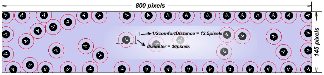
A typical C20 subway carriage used in Stockholm Metro is 46.5 meters in length and 2.8 meters in width. To control the model complexity, we select 1/3 of the carriage and scale down (with a mapping of 1 pixel ≈ 1.93 × 10⁻² meter) to 800 pixels long and 145 pixels wide, as shown in Figure 4. In this paper, we use a set E to denote all key properties that constitute the enclosed space of a C20 carriage.

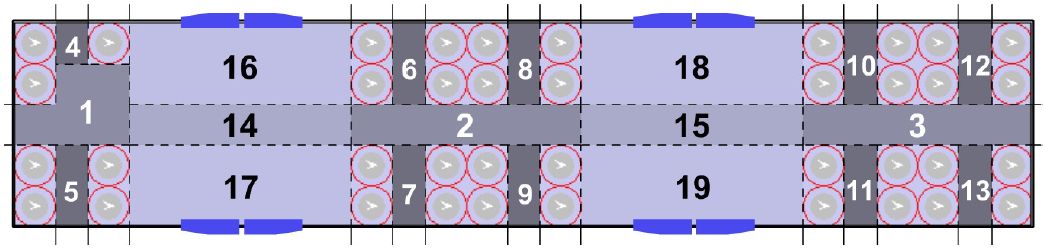
The manual zone partition (No. 1 ∼ 19) of the focused part of an SL C20 carriage.

The measurements of the simulated environment space E and the agent attributes p, q.
According to the standard seat distribution for C20 subway carriage used by Stockholm Metro as illustrated in Figure 2(b), there are 39 seats in that 1/3 part of an integrated carriage. Four doors situated on both sides divide the seats in a C20 carriage into 3 sections from left to right in general. In our model, all seats are supposed to be occupied by fixed passengers who do not stand up or move during the whole simulation process. Hence, some passenger behaviors, such as looking for seats and taking turns to sit, are excluded temporarily from our current study. By doing this, the variables in our simulations and experiments are simplified and become easier to control and analyze, because our research goal is to verify the validity of the proposed model instead of simulating the intact real world.
Under the consideration of applying both qualitative and quantitative methodology to the upcoming evaluations, the focused part of C20 carriage is partitioned to 19 zones belonging to 4 categories (corridor, seat, central, and doorway zone) as is shown in Figure 3.
Corridor zone: this category includes 3 areas (No. 1 ∼ 3). Passengers constantly pass them to look for comfortable positions, but few passengers like to stay still in these areas normally.
Seat zone: it includes 10 areas (No. 4 ∼ 13). They are located between seats that are facing each other. They are usually considered too narrow to hold any passengers unless there are way too many passengers in the carriage.
Central zone: two areas (i.e. No. 14 ∼ 15) belong to this category. When passengers are looking for comfortable positions, central area is probably the most crowded region, for people must walk across central areas to reach other types of areas.
Doorway zone: it contains 4 areas (No. 16 ∼ 19). They represent areas around the 4 doors in the focused carriage region. Doorway areas, together with central zones, tend to be the most preferable areas for passengers to stand in according to our observations.
2.2 Agent attributes
An agent An, (n=1,…,Nt) representing a passenger moves continuously via constant interactions with the environmental space and other agents; hence its status (a.k.a. attributes) may change along the time-line, making An at time-point t potentially different (from the perspective of embodied attributes) from that at the next time-point t +1. Due to the limitation of computerized simulation, we have to treat the concept of time in a discrete manner, but in reality, time is a continuous concept. We denote the n-th agent at time t as , which contains five attributes assembled in a seven-tuple array:
where Nt is the total number of agents in the predefined space; records the location (in form of a coordinate pair) of agent An at time t, as demonstrated in Figure 6(a); pn is a constant variable denoting the diameter of an agent represented in a solid circle (Figure 4); is the comfort distance of agent An at time t, representing the minimum distance which agents would like to keep between each other; denotes the current moving direction (a.k.a. facing angle) of agent ; and vn is the speed/velocity in which the agent An is moving at time t; we use to denote the zone where agent An locates at time t; and finally, the mobility variable is an integer indicating the maximum number of zone-transit actions allowed for agent An at time t. We will specify these attributes one after another in the following sections.
2.2.1 Agent diameter: pn
We have observed that the average hominine shoulder length is 80 centimeters, which is much longer than its width. For the sake of simplicity, we empirically stipulate that a passenger occupies a 70-centimeter-diameter rotundity if observed from a top-plan view. We then scale it down by the same ratio used in processing spatial data (cf. Section 2.1), resulting in a 36-pixel-diameter rotundity (i.e. pn = 36 as shown in Figure 4).
2.2.2 Dynamic comfort distance:
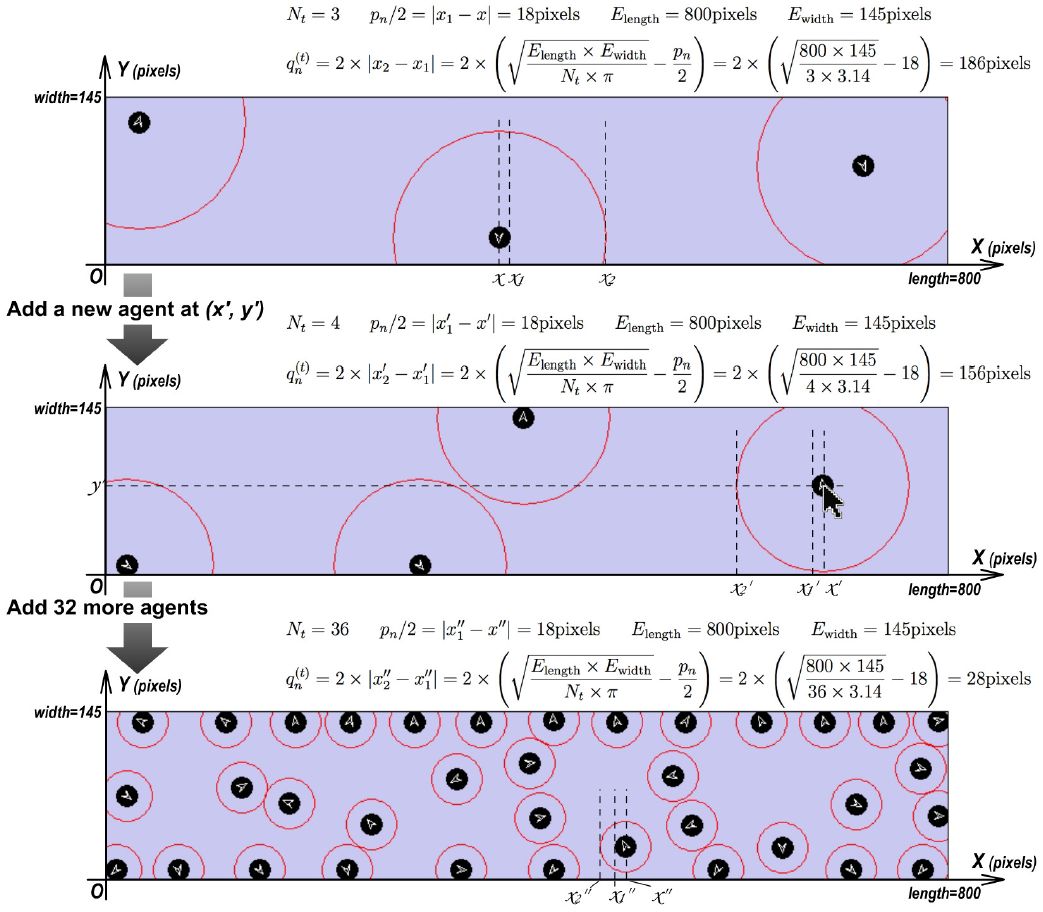
Some researchers (Holmes & Spence, 2004; Graziano & Cooke, 2006; Coello, Bourgeois, & Iachini, 2012) conceive“comfort distance”a protective buffer surrounding the body and prompting defensive actions, which is represented by highly integrated multisensory and motor processes in frontal-parietal and posteromedial areas (Ruggiero, Frassinetti, Iavarone, & Iachini, 2014; Iachini, Coello, Frassinetti, & Ruggiero, 2014). In real world, we observe that passengers tend to adapt this distance according to the number of passengers in the carriage. Thus, we apply the mechanism of automatic comfort distance adaptation (a.k.a. dynamic comfort distance): the comfort distance changes depending on the current number of agents in the simulated carriage; more agents lead to smaller comfort distance. We denote the length and width of the space as Elength and Ewidth respectively; provided that Nt agents exist at time t, the current comfort distance of each agent (i.e ) is calculated by
An example of applying this dynamic variations mentioned above to our model is given in Figure 5. We believe this mechanism makes our microsimulation model step closer to reflecting the dynamic characteristic of pedestrian movement in a subway carriage to a certain extent.
An calculation example of dynamic comfort distance : auto-adaptation according to Nt.
2.2.3 Agent moving direction:
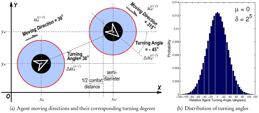
This attribute identifies an agent's current facing angle which may be any value from a finite-discrete set {0°,1°,…,358°,359°}, as illustrated in Figure 6. Since agents can only move ahead along their facing directions, the terms “ moving direction”, “ facing angle”, and “ orientation” essentially refer to the same attribute . If we informally compare the simulation procedure to a movie clip constituted by many consecutive frames, then each agent An on the t-th frame (with a facing angle ) will have to be assigned with a new moving direction (noted as ) for frame t +1. Constrained by the processing capability of the computer which runs our micro-model, we fix the update frequency Efreq (of agents’ moving direction and position) to approximately Hz (i.e. ≈ 30 milliseconds). Based on the fact that it becomes harder for a passenger to perform a larger-angle turn in an extremely short time-frame (30 ms), we simply select the relative turning angles (noted as ) for all agents obeying a Gaussian distribution [cf. visualization in Figure 6(b)]:
where denotes the probability that turning degree is selected and added to the t-th time-frame; parameter µ = 0° is the mean (or expectation) of the distribution; notation σ = 25 defines the scale (or span) of the distribution. The final value of σ is decided through a series of validations (similar to the evaluation approach introduced in Section 3.3.2) towards different candidate values. With the precedent definition of relative turning angle in Equation (3), we are able to compute the new agent moving direction with
where mod(a, b) denotes the remainder of the Euclidean division of a by b.

Illustration of agent turning angle that is selected obeying a discrete Gaussian distribution.
2.2.4 Agent moving velocity: vn
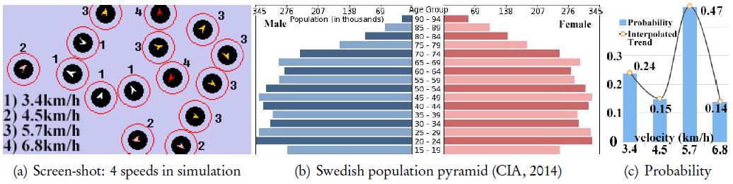
As is analyzed in (M. Q. Liu, Anderson, Schwartz, & Delp, 2008), biological human diversity is ubiquitous in real world; their preferred moving velocity is treated as an important aspect of diversity in our model. Although walking speed can vary greatly depending on a multitude of factors such as height, weight, age, fitness, and group size, specific studies (Samra & Specker, 2007; Rastogi, Thaniarasu, & Chandra, 2010) have found the average human walking speed is about 5.0 kilometers per hour (km/h); the pedestrian walking speeds range from 4.51 to 4.75 km/h for older individuals and from 5.32 to 5.43 km/h for younger individuals; a brisk walking speed can be around 6.5 km/h; and race-walkers can average more than 14 km/h. When evaluating our model with unsupervised machine learning techniques in Section 3.3, we normalize the time-consumption of model-execution and in-field observation respectively; therefore, the relative distribution of agent speed-levels turns out to be more important than the individual absolute speed-values.
According to the age-structure statistics of year 2014 from (CIA, 2014), Swedish population can be largely seen as a continuation of 5 age groups, the proportions of which [cf. Figure 7(b)] are 0∼14 yr: 17.12%, 15∼24 yr: 11.97%, 25∼54 yr: 39.30%, 55∼64 yr: 11.63%, and 64 yr+: 19.99%. During our in-field observations, we rarely see passengers aged 0∼14 yr who travel alone, hence we only consider 4 age-groups whose ratios are rescaled within [0,1]according to the aforementioned proportions respectively: 55∼64 yr: 0.24, 55∼64 yr: 0.15, 25∼54 yr: 0.47, 15∼24 yr: 0.14. For simplicity, we directly map the agents to those age-groups using 4 speed levels as illustrated in Figure 7(a): 1) agents with a white arrow have the slowest moving speed of 3.4 km/h(≈1.5 pixels/30ms); 2) agents labeled with a pink arrow move at a speed of 4.5 km/h(≈2.0 pixels/30ms); 3) agents with an orange arrow have a speed of 5.7 km/h(≈2.5 pixels/30ms); 4) the red-arrowed agents have a fastest speed of 6.8 km/h(≈3.0 pixels/30ms). These speed levels basically coincide with our in-field body-storming (Oulasvirta, Kurvinen, & Kankainen, 2003) activities, which probably simulate 4 different kinds of pedestrian walking speed resulting from 2 basic dimensions: age (young ↔ old) and gender (male or female). The initialization of agents follows a discrete probability distribution [Figure 7(c)], and the interpolated version of which coincide with a certain binomial distribution.

The heterogeneous agent moving speeds are mapped to groups of Swedish population.
2.2.5 Agent mobility index:
The initial values of agent mobility indices for all agents (i.e. ) are empirically defined as
which will be decreased upon zone-transit (Section 2.3.4) and increased upon active/passive comfort-distance violation (Section 2.3.5). When this variable reaches zero, the corresponding agent stops moving any more until its mobility index becomes positive again due to the violation of comfort distance.
2.2.6 Agent zone-location:
With respect to the zone partition in Figure 3, is assigned with the numerical label of the zone where the n-th agent stays at time t. Therefore .
2.3 Agent behaviors
The diverse behaviors of agents are consequences of their interaction with each other and the environment in which they are situated (Bonabeau, 2002). Based on the belief that agent's behavior depends on the role it currently plays, many common agent-based modeling approaches model agent behavior with a finite state machine, which perpetually loops through a list of roles (Ronald, 2007). However, the success of this approach requires macro-level understanding of the target “ecosystem”, while creating computational models of pedestrian behavior is usually difficult (Benenson & Torrens, 2004). Walking behavior is largely unconscious and unpredictable; sometimes it is hard to figure out why we take a particular path, which is one example of the so-called “emergent behavior”. As an essential property of any complex system, emergent behaviors are defined as “large-scale effects of locally interacting agents that are often surprising and hard to predict even in the case of simple interaction” (Boccara, 2010), which is uninterpretable by macro simulations. With this circumstance, authors of (Bar-Yam, 1997; Benenson & Torrens, 2004) supported microsimulation by claiming that 1) “the actions of the parts do not simply sum to the activity of the whole” and 2) “the behavior of the system cannot be simply inferred from the behavior of its components”. As such, we merely define several local-and-simple agent-level behaviors, as an integral part of our micro-model.
2.3.1 Moving forward
For any agent An whose mobility index mn is larger than zero at time t (i.e. ), it keeps moving along its facing angle at its pre-defined velocity vn (cf. Section 2.2.4). We examined qualitatively that agents with faster speed are willing to go through passages like zone No. 2. But agents with slower speed are apt to stay at their current locations and rarely go through passages; even if they are shoved in a passage, they would stop there and cause a so-called “traffic jam”.
2.3.2 Regular steering
Agent moving direction rotates a certain angle either clockwise or anti-clockwise stochastically every Efreq =30 milliseconds. The relative turning angle and absolute moving direction are calculated with Equation (3) and (4) respectively.
2.3.3 Wall avoidance
Agents are restricted to move in the subway carriage represented as a rectangle area; they should be capable of detecting the existence of a “wall” nearby and turn away from it. Concretely speaking, if an agent An collide into any part of the wall at time t, its facing angle will be immediately reset to the orthogonal direction against that wall, i.e.
2.3.4 Mobility decay
The behavior of mobility decay means that the mobility index will be decreased by one, as soon as its owner agent goes across the border of any zone (i.e. the dashed lines in Figure 3); it is formulated as
Because the agent stops moving upon , the main purpose of designing this behavior is to stabilize the simulation by making the model converge gradually. The global objective function that specifies the end point of micro-model execution is formally defined in Section 2.4.
2.3.5 Comfort distance violation
When an agent moves into another agent's comfort distance circle, they will stop moving forward and change moving directions instead (cf. Section 2.2.3) to maintain the comfort distance between each other. Namely, there should be no other agents within the comfort distance of a certain agent. Referring to Figure 6(a), between any 2 agents An and An′, the result of the following proposition must be maintained at all times:
Whenever the above constrain between agent and is violated, we will, at the next time frame t +1, update the mobility indices for both agents with the formula below, so as to boost their “motivation to walk” out of the comfort-distance collision.
2.3.6 Unaddressed agent behaviors
We intend to briefly present a small topic, in this section, on agent behavioral mechanisms (e.g. clustering, giving way, seat searching, and queuing) which are not yet considered as a part of our microsimulation and are, rightfully so, no part of the scope of this research. The clustering (a.k.a. cohesion) behavior makes agents tend to stick together in family/friend relations, which in practice can be implemented by constraining the maximum distance allowed between any two agents within the same cluster. An-other behavior of cooperation between agents is giving way, which stipulates conditions such as letting others off first before getting on and making room for others to pass through corridor zones. When simulating the seat searching behavior, agents may be attracted to take the seat that has more empty seats around it. Unlike the “random walk” of agents in an enclosed moving carriage, getting on/off the carriage turn out to be more of an organized queuing behavior, which can be implemented in various ways. It is notable that if these unaddressed agent behaviors are adopted, further assessment of design schemes will be influenced accordingly.
2.4 Simulation process and global objective function
A valid micro-model execution must embody 3 parts/stages as shown in Figure 1: initialization, “free-lancing”, and convergence. The initialization usually requests presetting interior artifacts (e.g. seats and handrails), existing agents (i.e. agents that are placed at certain locations inside the carriage), and entering agents (i.e. agents that are going to enter the carriage). Throughout this paper (cf. Figure 3 and Table 1,2), notation “a:b ” (e.g. 16:2) represents placing b (e.g. 2) agents in zone a ∈{1,…,19} (e.g. 16); and “a′-b′” (e.g. 17–3) means b′ (e.g. 3) agents are queued outside of doorway zone a′∈{16,…,19} (e.g. 17), waiting to enter the carriage via that doorway at the beginning of “freelancing” phase.
Real data collected from in-field observation.
| di | Initial Status (entering|existing passengers) | Real-data Dimensions (i.e. di,1, di,2,…, di,23) |
| d1 | 17-01,19-03|16:1,17:2,18:1,19:1 | 1,0,0,0,0,0,0,0,0,0,0,0,0,1,1,2,1,2,1,08,0,1,0 |
| d2 | 17-03,19-00|14:1,16:3,17:2,18:2,19:4 | 0,1,0,0,0,0,0,0,0,0,0,0,0,2,1,1,2,4,4,12,4,3,0 |
| d3 | 16-01,18-03|9:1,14:3,15:3,16:4,17:3,18:2,19:2 | 1,1,1,0,0,0,0,0,1,0,0,0,0,3,3,2,4,3,3,18,1,1,0 |
| d4 | 16-02,18-05|1:1,14:3,15:3,16:4,17:2,18:4,19:3 | 3,2,3,0,0,0,0,0,0,0,0,0,0,4,4,3,3,2,3,20,3,1,1 |
| d5 | 16-07,18-05|1:1,2:2,14:3,15:2,16:5,17:5,18:5,19:3 | 4,2,3,0,0,1,0,0,0,0,0,0,0,5,7,4,2,6,4,31,6,3,2 |
| d6 | 17-09,19-08|1:2,2:4,14:2,15:2,16:7,17:3,18:4,19:4 | 3,3,2,0,0,1,1,0,0,0,1,0,0,6,7,6,5,4,6,28,3,1,1 |
| d7 | 16-10,18-06|1:4,3:1,4:1,7:1,14:4,15:2,16:5,17:4,18:4,19:4 | 3,2,2,0,0,0,1,0,0,0,0,0,0,5,9,7,6,4,7,30,7,4,3 |
| d8 | 17-08,19-10|1:2,2:2,3:2,4:1,8:1,14:2,15:2,16:5,17:2,18:6,19:5 | 4,4,3,1,0,0,0,1,0,0,0,0,0,5,8,3,8,7,4,35,0,3,5 |
| d9 | 17-11,19-13|1:2,2:2,3:1,6:1,8:1,14:3,15:3,16:4,17:3,18:2,19:3 | 2,4,2,0,1,0,0,0,1,1,0,0,0,6,8,6,5,5,8,40,3,3,4 |
| d10 | 16-10,18-11|1:3,2:4,3:2,6:1,7:1,10:1,14:5,15:4,16:5,17:4,18:4,19:5 | 4,6,3,0,0,1,1,1,0,1,0,0,0,8,9,8,7,5,6,46,4,6,5 |
We borrow the term “freelancing” to describe the autonomous and lengthy process that constitutes diverse interplay among agents and their surroundings. It is crucial that this process should not be intervened in any way until convergence is reached; hence both emergent behavior (Boccara, 2010) and self-organisation (Helbing et al., 2001; Ronald, 2007) can occur unexpectedly. Different from emergent behavior, self-organisation occurs when the system organises itself into a more-ordered state, with no central control.
The model execution ends at the time point t, when agents keep relatively stable in the whole simulated carriage area. This global steady state or convergence implies that there is a global objective function which is of key importance to every single simulation; and with the same notation convention as in previous Sections 2.1, 2.2, and 2.3, this objective function (a.k.a convergence target) is formulated as
where fE,A,t′ (t )is the overall spatio-temporal agent entropy at time point t, which measures the accumulated dynamic uncertainty of all agents over an empirical time period of t′ (i.e. from t − t′ +1 to t ); it increases when the simulated space is closer to random/chaos, and decreases when it becomes less randomized/chaotic. The model converges when there are no agents traversing across different areas within t′, i.e. fE,A,t′ (t )=0; and parameter t′ tunes our model's tendency to converge: the larger it grows, the more difficult to minimize Equation (9).
3. Model evaluation and verification
In the previous chapter, our microsimulation prototype for modeling passengers in a subway carriage is described from the aspects of environment space, agent attributes, agent behaviors, and the objective function. Following the development of the prototype model, it is necessary to assess and explore its practical usefulness. However, most previous researches looked at different qualitative methods (Axelrod, 1997; Kelton & Law, 2000; Tobias & Hofmann, 2004) for deciding whether a pedestrian model was appropriate; and so far, little quantitative research has been undertaken into evaluating micro-models designed to “mimic” a specific activity. Inspired by the recent advancement in the hotspot research areas of generic machine learning and feed-forward neural networks, we propose a novel quantitative-oriented approach to verify the maturity and feasibility of our pedestrian micro-model; it is implemented by training a complex nonlinear Single-hidden-Layer Feed-forwardNetwork (SLFN) (Rumelhart, Hinton, & Williams, 1986) with labeled simulation data, and then measuring the learned SLFN's generalization and discrimination performance on predicting the real data collected from in-field observations. In the following sections, we will consecutively elaborate on real data collection, simulation data generation, quantitative model evaluation, and a qualitative case study.
3.1 Real data collection: In-field observation
The purpose of in-field data collection is to gather 10 real datasets by observing 10 “valid” pedestrian flow processes within a C20 carriage operated by Stockholm Lokaltrafic (SL). A valid pedestrian flow process starts from the time when passengers, who intend to get off the carriage upon arrival at a subway station, have all gone out of the carriage. Similar to the term “existing/entering agents” defined in Section 2.4, the initial passenger distribution in the carriage is recorded in the form of “a:b ” (Table 1) implying b passenger(s) in zone a; and passengers queuing outside the carriage doors are noted as “a-b ” (Table 1) implying that b passenger(s) will enter through doorway zone a. The newly entered passengers orientate themselves and coordinate with original passengers in the carriage to look for their own comfortable positions. And observation can be counted as a “valid” one only when 1) no passengers sit down, and 2) no passengers walk to the other 2/3 C20 carriage. The pedestrian flow process ends at the time when all passengers stay relatively stable in the carriage, meaning there are no passengers traversing across different areas within an empirical time period.
For the i-th valid observation (i.e. “real data” di in Table 1), we use di, j (j =1,…,19) to denote the number of passengers in the j-th zone after the end-point is reached (a.k.a. “static features” in Table 1), and use di, j (j =20,…,23) to represent the “dynamic features” that basically reflect important characteristics of passengers’ movement; they denote the time needed to reach the end point (di,20), number of passengers that once went from zone 14 to 15 (di,21) or the other way around (di,22), and the number of passengers who are still moving in the end (di,23). We construct a matrix D to denote the entire real datasets:
where di is a row vector denoting the i-th real-world data, i.e. di =[di,1,…, di,23]. We also represent the observation categories/IDs with a matrix G:
With these notation definitions, we can jointly represent the real data with IDs (i.e. labeled testing data in Section 3.3) in the form of ℵ = {(di, gi )|di ∈ ℝ23, gi ∈{0,1}10, i =1,…,10}.
3.2 Simulation data generation: Micro-model execution
Based on the real data collected from in-field non-intrusive observation, our micro-model is executed in order to gain 100 valid sets of simulation data, which will be “compared” with real data using machine learning techniques. The micro-model execution exactly follows the 3-stage process (i.e. initialization, “freelancing”, and convergence) specified in Section 2.4. For each real data di, we initialize our model with the same “initial status (entering|existing passengers)” as in Table 1, and run (i.e. “freelancing”) it until convergence for 10 times. The reason of multiple simulations per real case is the basic belief of microsimulation theory: “what is valid should be the aggregated overall result from multiple micro-model executions instead of the separate result from one single execution” (Axelrod, 1997). Ultimately, weget10×10=100 simulative data , each of which also consists 23 feature dimensions referring to the same static/dynamic characteristics as in real data. Table 2 presents portions of the simulation dataset; it is mathematically denoted as , in which we have equivalent [as Equation (10) and (11)] definitions of
Partial simulation data samples generated from 100 valid micro-model executions.
| Model Initialization (entering|existing agents) | Features of Simulation Data | |
| 17–01,19–03|16:1,17:2,18:1,19:1 | 1,0,0,0,0,0,0,0,0,0,0,0,0,0,0,4,0,3,1,05,00,1,1 | |
| 17–01,19–03|16:1,17:2,18:1,19:1 | 1,0,1,1,0,0,0,0,0,0,0,0,0,1,0,1,1,0,3,10,00,0,4 | |
| 17–01,19–03|16:1,17:2,18:1,19:1 | 1,0,1,0,0,0,0,0,0,0,0,0,0,1,0,3,1,1,1,13,00,2,3 | |
| 17–01,19–03|16:1,17:2,18:1,19:1 | 1,0,3,1,0,0,0,0,0,0,0,0,0,0,0,1,1,1,1,18,04,4,4 | |
| 17–01,19–03|16:1,17:2,18:1,19:1 | 1,0,2,1,0,0,0,0,0,0,0,0,0,1,0,1,1,1,1,10,02,3,5 | |
| 17–01,19–03|16:1,17:2,18:1,19:1 | 1,0,3,1,0,0,0,0,0,0,0,0,0,0,0,1,1,1,1,09,03,3,4 | |
| 17–01,19–03|16:1,17:2,18:1,19:1 | 1,0,3,1,0,0,0,0,0,0,0,0,0,0,0,1,1,1,1,10,02,2,4 | |
| 17–01,19–03|16:1,17:2,18:1,19:1 | 1,0,1,1,0,0,0,0,0,0,0,0,0,0,0,1,1,1,3,08,01,1,3 | |
| 17–01,19–03|16:1,17:2,18:1,19:1 | 1,0,0,0,0,0,0,0,0,0,0,0,0,0,0,3,1,3,1,05,00,1,2 | |
| 17–01,19–03|16:1,17:2,18:1,19:1 | 1,0,0,0,0,0,0,0,0,0,0,0,0,0,0,4,0,1,3,07,00,1,1 | |
| 17–03,19–00|14:1,16:3,17:2,18:2,19:4 | 1,0,1,0,1,0,0,0,0,0,0,0,1,0,0,3,4,2,2,23,05,5,0 | |
| 16–01,18–03|9:1,14:3,15:3,16:4,17:3,18:2,19:2 | 1,1,1,0,1,0,0,0,0,0,0,0,1,1,2,5,1,4,4,27,02,3,1 | |
| 16–02,18–05|1:1,14:3,15:3,16:4,17:2,18:4,19:3 | 3,2,2,0,0,1,0,0,0,0,0,1,0,4,4,2,3,2,3,43,05,1,1 | |
| 16–07,18–05|1:1,2:2,14:3,15:2,16:5,17:5,18:5,19:3 | 3,3,2,0,0,1,0,0,1,0,1,0,1,5,5,4,3,6,3,46,07,2,2 | |
| 17–09,19–08|1:2,2:4,14:2,15:2,16:7,17:3,18:4,19:4 | 4,2,3,0,1,2,0,0,0,1,0,0,0,6,5,7,5,6,3,47,05,2,1 | |
| 16–10,18–06|1:4,3:1,4:1,7:1,14:4,15:2,16:5,17:4,18:4,19:4 | 3,1,2,1,0,1,0,1,0,1,0,0,0,4,7,8,6,5,6,52,10,3,4 | |
| 17–08,19–10|1:2,2:2,3:2,4:1,8:1,14:2,15:2,16:5,17:2,18:6,19:5 | 3,5,3,0,2,0,1,0,0,1,0,0,1,5,6,4,6,6,5,56,01,3,5 | |
| 17–11,19–13|1:2,2:2,3:1,6:1,8:1,14:3,15:3,16:4,17:3,18:2,19:3 | 2,5,3,0,0,1,1,0,1,0,0,1,1,7,5,6,5,5,6,63,04,2,4 | |
| 16–10,18–111:3,2:4,3:2,6:1,7:1,10:1,14:5,15:4,16:5,17:4,18:4,19:5 | 5,6,2,0,2,1,1,0,1,0,1,0,1,7,7,8,6,6,6,69,04,5,5 |
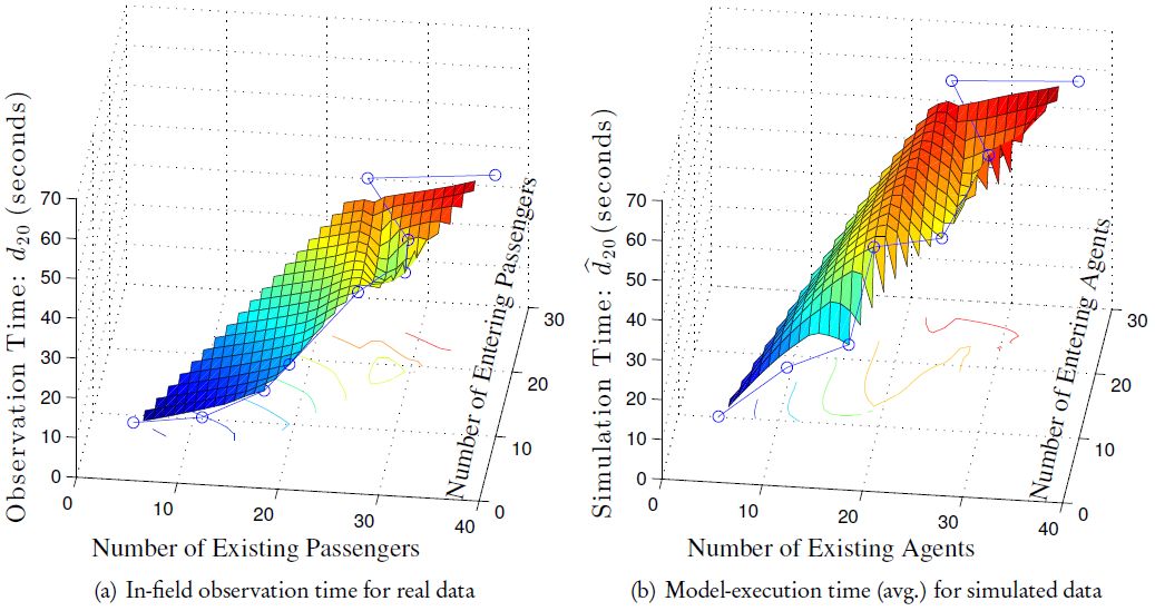
To empirically investigate the relationship between model-execution time (or “in-field observation time” for real data) and existing/entering agents (or “existing/entering passengers” for real data), we visualize the values of in Figure 8(b) and di,20 in Figure 8(a) as a function of existing and entering agents/passengers. The model-execution time in Figure 8(b) for each parameter combination (i.e. existing and entering agents) is averaged over 10 “valid” simulations with the same presetting of existing-entering agents. The visualizations in Figure 8 show that both real and simulated pedestrian models operate in linear time with respect to either existing or entering individuals; this is to be expected as there are no complex interactions. Hence in both cases, the relationship between the add-up density (existing +entering individuals) and run time becomes polynomial. However, the time-consumption of simulation grows faster than that of real-world observation, which is probably caused by the fact that passengers are more efficient (than agents) in resolving conflicts by possessing context-awareness and global-sensitiveness; this discovery also coincides with the efficiency analysis in (Ronald, 2007).

The observation/simulation time (blue line) and the corresponding cubic interpolations (3D surface) as a function of existing and entering passengers/agents.
3.3 Quantitative model evaluation: Machine learning
The primary goal of this quantitative evaluation is to answer the question that whether our proposed micro-model can precisely reflect and predict the real passenger flow in a subway carriage; and we tackle this question by estimating the similarity level between real and simulation data. Intuitively, we could calculate the mean within each simulation group, and compute a summation over all deviations (e.g. absolute, squared error, etc.) per variable. Furthermore, we could also apply weights on different variables (equivalent to a linear model), since they might not be equally important. We empirically tested those evaluation methods and found out that 1) the simple averaging over 10 raw simulations may lead to faulty conclusions as the mean statistics are not guaranteed results from our simulations and might just represent a situation that will never take place in the simulated environment; 2) the unbiased treatment on different variables seems awkward since they (e.g. execution time and traversing agents , ) clearly impose a different unit that will hamper the measurement via their varying amplitude; 3) even if different coefficients are utilized to weigh all 23 variables, the manual selection and optimization of weights [e.g. via grid search (Hinton, 2012; Cao et al., 2014a; Cao, Huang, & Sun, 2014b)] might just be yet another challenging and time-consuming work; 4) there is no guarantee that linear weight combination works better than a nonlinear version.
To address the above problems commonly seen in quantitative model-evaluation approaches, we pro-pose to use the state-of-the-art machine learning methods to evaluate the effectiveness of our micro-model; in particular, SLFNs are our major focus. Extreme Learning Machine (ELM) (G.-B. Huang, Zhou, Ding, & Zhang, 2012; G. Huang, Huang, Song, & You, 2015; G.-B. Huang, 2015), as a novel learning algorithm originated from SLFNs at the very beginning, is well-known for its simple architecture with proven potential in solving classification and regression problems; ELM also tends to reach both the smallest training error and the smallest norm of output weights, requiring less human intervention and supervision than other supervised learning algorithms (G.-B. Huang et al., 2012). As a result, we train an ELM network from labeled simulation data (cf. Section 3.3.1), use the trained network to predict the classes/labels of real data (cf. Section 3.3.2 and 3.3.3), and report the model's approximation ability from aspects of accuracy, standard deviation, precision, recall, confusion matrix, and receiver operating characteristics (ROC) graph (Fawcett, 2006).
3.3.1 Supervised training on simulation data
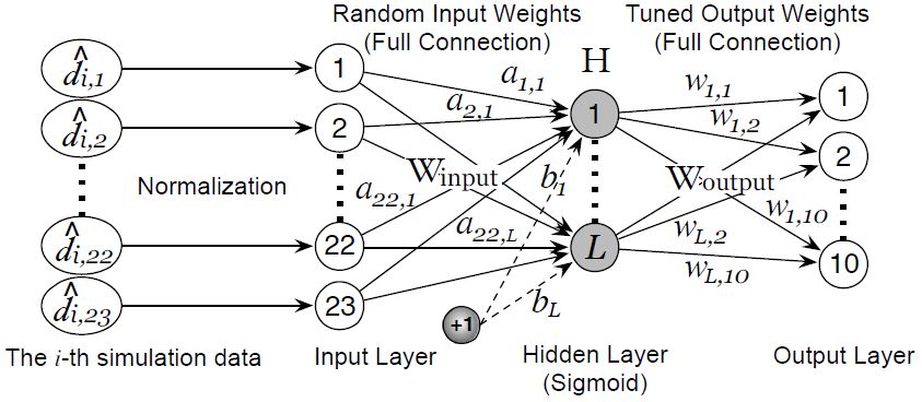
ELM can conveniently approximate complex nonlinear mappings directly from the input simulation data. As shown in Figure 9, it has 3 essential layers (input, output, and hidden layer) and 3 fundamental parts (random projection, nonlinear transformation, and linear combiner) (Cao, Huang, & Sun, 2015). In a nutshell, the hidden layer maps the input space (23 dimensions in our case) onto a new space (L dimensions) by performing a fixed nonlinear transformation with no adjustable parameters, while the output layer behaves like a linear combiner on the new space. We simply use the sigmoidal activation due to its proved universal approximation and classification capability (G.-B. Huang et al., 2012), thus the activation function of the i-th hidden node is
where the input weights Winput ∈{ai, bi }i=1…L are randomly generated obeying any continuous probability distribution (G.-B. Huang et al., 2012). The transformed feature space H is defined as
where is called the activation function of the i-th hidden neuron; and row vector is the output vector of the hidden layer with respect to the j-th input vector; in other words, hj maps the raw feature to L dimensions. The row vectors of are in full connection (weighted by Woutput in Figure 9) with 10 output nodes representing 10 simulation classes. Principally, Woutput ∈ RL×10 = [w1,…,wL]T can be learned with any supervised learning algorithm; and we follow (G.-B. Huang et al., 2012) to tune Woutput because of its fast training speed and good generalization ability:
where is defined in Equation (12); small positive values are added to the diagonal of HHT to improve the stability and generalization ability of the resulting solution; the user-specified parameter C is a tradeoff between the distance of the separating margin and the training error (G.-B. Huang et al., 2012). After all the nonlinearities in the hidden layer are fixed, the output layer behaves like a linear combiner. When the number of training samples is larger than that of hidden nodes, the second solution should be applied to reduce computational costs.

The structure of a typical ELM network with one hidden layer (with L nodes), one input layer (with 23 nodes), and one output layer (with 10 nodes representing 10 categories).
3.3.2 Predicting labels of real data: Unified multinomial classifier
It is often recommended in machine learning practice to normalize feature values per dimension; and in our real and simulation data, all feature values except di,20 and (time measures) reside in the region of [0,10], therefore we normalize them to [0,10]respectively to eliminate inordinate significances. Since the unified ELM classifier (G.-B. Huang et al., 2012) naturally permits the use of more than two classes, we use the following multinomial/multiclass decision function, when predicting the labels for real data di,I ∈{1,2,…,10}:
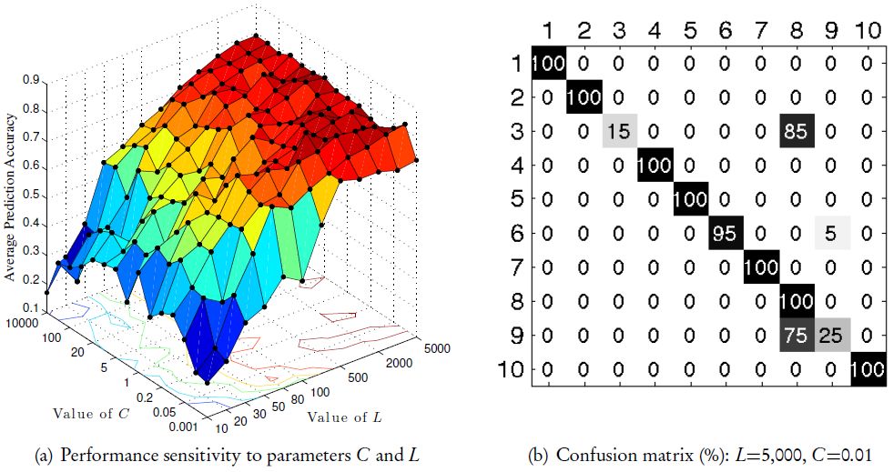
where o denotes one of the label IDs. Inspired by (Ghanty, Paul, & Pal, 2009) and (Cao et al., 2014a), we carried out a grid search (Hinton, 2012; Cao et al., 2014a) for optimal (C, L)parameter combinations; we tested 15 values of C ∈{0.001,0.01,0.05,0.1,0.2,0.5,1,2,5,10,20,50,100,1000,10000} and 12 different values of L ∈{10,20,30,50,80,100,200,500,1000,2000,3000,5000}, leading to a total of 180 trials/tests. According to the analysis in (Cao, Huang, Sun, et al., 2015; Cao, Huang, & Sun, 2015), the Moore-Penrose pseudo-inverse (Rao & Mitra, 1971) to tune Woutput [Equation (15)] can lead to numerical instabilities if the training sample matrix is not full rank, which is unfortunately very often the case for real-world data (Miche, Van Heeswijk, Bas, Simula, & Lendasse, 2011). Because the parameters for the hidden nodes are randomly generated, the feature mapping matrix (i.e. H) does not stay the same given identical training and testing data, making the prediction accuracy of a single trial different from other trials. Although this kind of performance variance becomes acceptable and controlled within certain limits by adding in Equation (15), it is still necessary to carry out groups of trials and calculate the average performance; for this reason, each score in Figure 10(a) were averaged over 20 trials.

The evaluation results obtained via an unified multinomial classifier: (a) the performance sensitivity obtained via grid searching; (b) the class-wise confusion matrix of prediction accuracy.
From Figure 10(a), we can see that good classification performance can be achieved as long as L is relatively large (without significant relevance to C), which helps us to evaluate our model easily and effectively by avoiding tedious and time-consuming parameter tuning. The best average prediction accuracy (84%) is obtained at L=5,000 and C =0.01, we thus drill down that case to per-category classification behavior by presenting the corresponding confusion matrix in Figure 10(b); it is apparent that the 3rd and 9th real data get the worst scores because they are mostly confused with the 8th class.
3.3.3 Predicting labels of real data: One-vs.-all binary classifiers
Although the unified multinomial classifier indicates that our micro-model is capable of approximating over 80% real-world pedestrian flow cases, it somehow failed to distinguish a few cases, which maybe a consequence of the difficulty in training a universally functional network for all classes based on such a limited set of training/testing samples. As a consequence, we naturally think of the one-vs.-rest (a.k.a one-vs.-all) strategy (Hsu & Lin, 2002) that trains a single binary classifier per class, with the samples of that class as positive samples and all other samples as negatives [cf. Equation (18)]. This strategy requires the k-th binary classifier to possess only one output node that produces one real-valued confidence score [i.e. scoring function f(k)(·)]:
where •(k) is the corresponding notation (as in Section 3.3.1 and 3.3.2) for the k-th classifier; and is a single-element vector because there is only one node in the output layer (cf. Figure 9) of a binary classifier. We further define the label/class matrix for the k-th classifier in a slightly different way from Equation (12):

We once again use the manual grid search strategy to select the optimal parameter set (L,C ) for each network/classifier; and to cope with performance variance, we train and test each binary classifier for 200 times from scratch, expanding the number of testing samples to 2,000 in a way. Unfortunately, the simulation and real data are rather imbalanced in that they contain only 10% positive samples, the networks can be very sensitive to the class distribution and might be misleading in some way (He, Garcia, et al., 2009). In our case, each binary classification problem consists of 10% positive class and 90% negative class; any dumb algorithm could easily achieve 90% prediction accuracy by putting all the testing samples into the negative class; the overall accuracy of 90% looks quite satisfactory, but the accuracy of the minority class being actually 0% should be emphasized. To deal with this kind of imbalanced data, we follow the improvement discussed by Zong, Huang, and Chen (2013), who introduced a straightforward solution of associating a higher C value to the minority class. Concretely for the k-th classifier, we define an 100×100 diagonal matrix Ω(k) associated with every simulation/training sample ; specifically if belongs to a minority class (i.e. positive class in our case), the associated weight should be relatively larger than others. The detailed means for defining the specific weight for each sample can be found in (Zong et al., 2013). Without losing generalization ability, the output weight matrix of the k-th binary classifier is trained with a formula adapted from Equation (15):
where Hk denotes the feature space of the k-th network/classifier, which is calculated with Equation (14); Lk and Ck are the classifier-specific parameters that need to be selected by us via grid search activities. We report the optimal parameters (Lk and Ck ), average prediction accuracy (Mean Acc.), and standard deviation (Dev.) of accuracies in Table 3, in which the highest score(s) is indicated in bold; the second best one(s) is noted with an asterisk∗; and the worst score(s) is underlined. The first and foremost conclusion drawn from Table 3 is that the mean accuracy of all 10 binary classifiers reaches 94.4%, greatly prevailing the best accuracy achieved (merely 84%) by the unified multinomial classifier (Section 3.3.2). From accuracy and stability (standard deviation) perspectives, the 4,5,7,8,10-th categories reach competitive performances, which implies that our micro-model can unambiguously simulate those 5 corresponding situations. Although the accuracies for class 1,3, and 9 appear inferior than that of others, they all surpass 87% without exception.
Parameters and measures of 10 one-vs.-rest binary classifiers (200 trials); the scores labeled with bold, asterisk, and underline represent the best, 2nd best, and the worst results respectively.
| Parameters & Measures | Class. k=1 | Class. k=2 | Class. k=3 | Class. k=4 | Class. k=5 | Class. k=6 | Class. k=7 | Class. k=8 | Class. k=9 | Class. k=10 | Mean |
| Lk | 103 | 102 | 500 | 103 | 2,000 | 200 | 200 | 103 | 50 | 500 | N/A |
| Ck (baseline) | 106 | 103 | 102 | 103 | 103 | 102 | 102 | 1 | 10 | 102 | N/A |
| Mean Acc. | 0.879 | 0.916 | 0.897 | 0.996∗ | 0.991 | 0.906 | 0.992 | 0.998 | 0.872 | 0.996∗ | 0.944 |
| Dev. | 0.074 | 0.036 | 0.015∗ | 0.021 | 0.029 | 0.037 | 0.027 | 0.012 | 0.074 | 0.02 | 0.034 |
| Precision | 0.852 | 1 | 0.1 | 1 | 0.942 | 0.643 | 1 | 0.985∗ | 0.291 | 1 | 0.781 |
| Recall | 0.799 | 0.16 | 0.005 | 0.965 | 0.97∗ | 0.135 | 0.92 | 1 | 0.195 | 0.955 | 0.61 |
Usually prediction accuracy is widely used to measure the effectiveness of a classifier; but as mentioned previously, in presence of imbalanced data, this metric may just fail to provide adequate information on the comprehensive performance. To give more insight into the accuracy obtained within each class in lieu of the accuracy of all the samples, we also evaluate the performance with precision and recall; precision is the rate of true positives (noted as t p) from all retrieved positives given by the algorithm while recall gives the rate of t p from all the positives in the dataset. For our case, we execute each network/classifier for 200 times, thus we use the following equations to compute the macro-average precision and recall for each class:
where for the i-th trial/execution, t pi denotes the number of samples belonging to positive class that are correctly classified; f pi is the number of samples that are incorrectly classified as being of positive class when actually they belong to a negative class; f ni represents the number of samples that are incorrectly classified as belonging to negative class when in fact they belong to positive class. The precision and recall scores are shown in the lower part of Table 3, from which we find that the mean precision score (78.1%) over 10 classes is much superior to the mean recall score (61%); nevertheless, both of them are significantly better than random guesses (i.e. 50%), indicating that our micro-model turn out to be generally discriminative when simulating minor situations. Ideally, we expect to make both precision and recall simultaneously as high as possible, however they are inversely related (Jizba, 2000), which means that we can only struggle to achieve a better compromise (e.g. Class 1, 4, 5, 7, 8, and 10 in Table 3) between them. On imbalanced dataset, either low precision or recall score may bring down the overall accuracy, but only within a certain limit (e.g. Class 2, 3, 6, and 9 in Table 3). Moreover, the inferior precision and/or recall scores for Class 3, 6, and 9 might just resemble and explain the results shown in Figure 10(b).
To provide a comprehensive visual illustration of the performance for each binary classifier, we also present ROC graphs (Fawcett, 2006) in Figure 11(b)∼(i), where a classifier corresponds to a point. As demonstrated in Figure11(a), x-coordinate of the point represents false positives rate(f pi /#Negative Sample) and y-coordinate represents true positives rate (t pi /#Positive Sample), so that classification results for both positive and negative class are perceivable with a single point. In other words, precision and recall are essentially a way of describing one single point on the ROC curve; and the performance exhibited by ROC graph is independent of class distribution (Zong et al., 2013). In Figure 11(a), the classifier denoted by point Z(0,1) is the optimal classifier, which can classify all samples correctly in both positive and negative class; classifier P(0.3,0.8) achieves 80% accuracy for positive class and 30% accuracy for negative class; the diagonal points, such as B, C, and D, represent random classifiers that generate random guesses about the sample label. On the other hand, points below the diagonal (e.g. yellow points) are in no way bad classifiers; they are actually consistent to the symmetric points within the upper triangle and can be obtained by reversing the label sign of each sample. Hence, the upper triangle rather than the lower triangle is of our interest. In short, for a certain category/class of passenger flow [Figure 11(b)∼(i)], the larger the green shadowed area is, the better our micro-model is capable of simulating that very category. In this way, we can not only estimate the overall and per-class simulation quality, but also easily rank all simulated cases by their level of simulation difficulty (e.g. from easy to hard): Class 4,8,10⇒7⇒5⇒2⇒1⇒6⇒9⇒3.
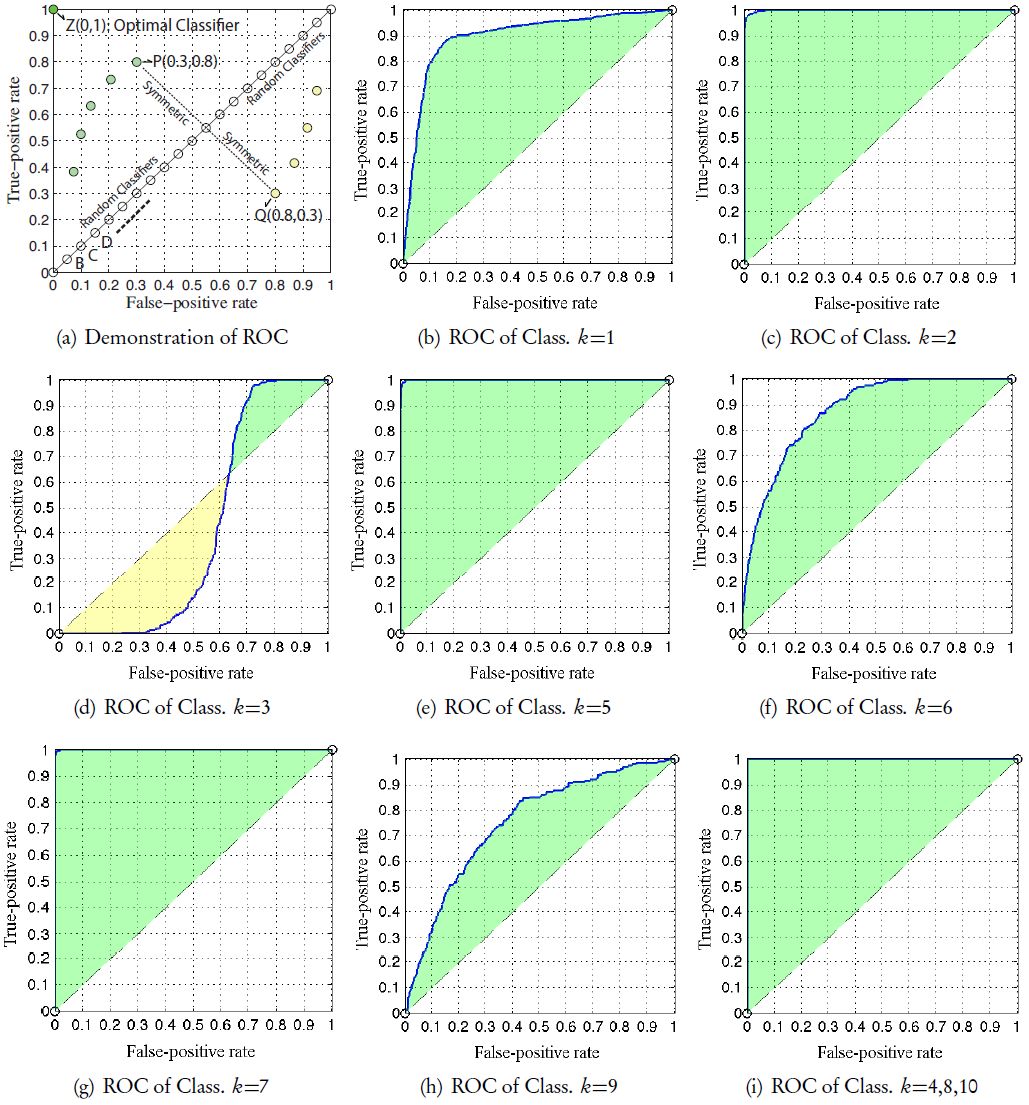

The quantitative evaluation results using receiver operating characteristics (ROC) graph:
3.4 Qualitative case study: Interior seat layout
Have validated simulation capability based on the typical seat arrangement of SL C20 subway carriage, designers could hereafter apply our micro-model to subway carriage design activities in various ways. As a lightweight example, we will present how we qualitatively evaluate different interior seat distributions using our micro-model. The case study methodology (Kitchenham, 1997) will be adapted in this section, which involves testing a model on different design candidates with a set of predefined lightweight assessment focuses.
In order to support on-demand agent creation, we optimize our source code in a way that an agent can be added at the very position where a mouse click occurs, which gives us the maximum possibility and flexibility to simulate different scenarios in which passengers enter the subway carriage. For instance, we could simulate the burst-out behavior of passengers by putting new agents one by one at certain locations where the doors are supposed to be; we could also add agents at some odd positions, for example directly in front of another agent, to see how they would react against the artificially created problematic situations.
3.4.1 Problems of the existing seat layout
In the course of both in-field observation and micro-model simulation, we have observed some problems caused by the existing seat layout in SL C20 carriage. As Figure 12 illustrates, people are not willing to traverse between the left and right part of the carriage; if too many people enter the carriage from the right sub-carriage door (18), the over-crowding incident tends to emerge in the right sub-carriage while the left sub-carriage remains relatively empty. We refer to this problem as “left-right sub-carriage imbalance”. Another problem with the existing seat setting in SL C20 subway carriage is called “doorway jam” (Figure 13), which occurs because passengers who decide to stand beside the doors have less possibility/willingness to leave these doorway areas. Even if new passengers shove them, they temporarily move a little and then return to original positions when possible; and it might directly reflect the fact that overcrowding incidents often happen in doorway areas in real life.
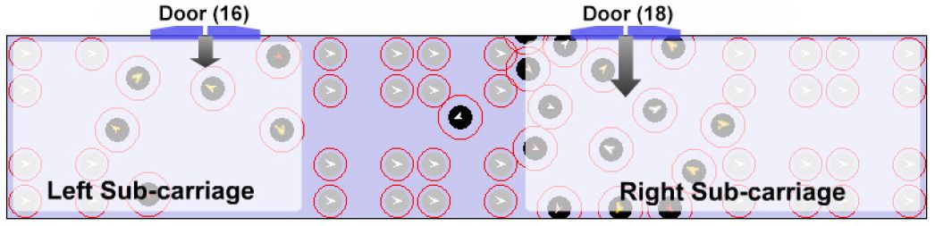

A screen-shot of “left-right sub-carriage imbalance” in the SL C20 subway carriage.
3.4.2 Analysis of a new seat layout
Observing the SL C20 subway carriage, we find passengers tend to stand along the wall in a row next to each other. So we assume that keeping areas near walls clear by removing the seats from those areas may contribute to utilizing space efficiently and satisfying passengers easily. A new form of seat distribution (Figure 14) is therefore designed and tested with our micro-model. There are 21 seats placed in the middle of a carriage with 4 aisles between them; and for simplicity, all seats are occupied by stationary passengers during the whole simulation process. It is delightful that there are no longer “left-right sub-carriage imbalance” or “doorway jam” problem observed in the carriage with the new seat layout, in which the newly entered passengers can unimpededly walk to other parts of the carriage. They would like to look for comfortable positions within the entire carriage and do not prefer gathering in the doorway area any more.

A screen-shot of “doorway jam” phenomenon in the SL C20 subway carriage.

A new design of seat layout by emptying wall areas in the SL C20 subway carriage.
However, a few new problems are brought forward by the new seat distribution. The first new problem is “pivot blocking”, meaning that passengers with lower moving speed sometimes block the pivot of pedestrian flow. This phenomenon becomes even more serious with the new seat distribution. As soon as pivot passages are blocked by one or more agents, it is rather difficult for other agents to diffuse between upper and bottom part of the carriage, as shown in Figure 15. The new seat layout is also problem-prone in the sense that passengers who will get off from the other side (upper/bottom) of the carriage must traverse one of the pivots.
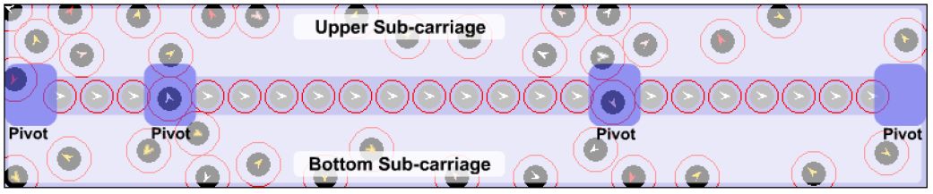

An example of “pivot blocking” in the SL C20 carriage with the new seat distribution.
The 21 seats in the new layout actually create a “wall”, separating the whole carriage into 2 narrow spaces: “upper sub-carriage” and “bottom sub-carriage” (Figure 15), in which passengers with lower moving speed tend to block the horizontal way. With the existing SL seat setting, when somebody gets in the horizontal way, passengers have to detour vertically and continue to walk horizontally; we call this phenomenon “vertical detour difficulty”. In the new seat layout, as observed from Figure 16, the vertical detour space becomes smaller because of the “wall” created by seats; hence a so-called “left-right sub-carriage imbalance” problem may emerge due to frequent “vertical detour difficulty”.
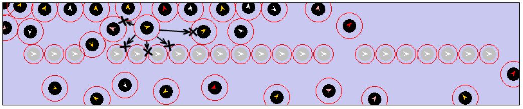
The “left-right sub-carriage imbalance” problem caused by “vertical detour difficulty”.
Another obvious disadvantage with the new seat setting is that there are fewer seats (21 seats) than the existing SL C20 seat layout (39 seats); thus the existing layout appears to be better in that it is capable of offering more passengers a comfortable trip. There are of course other advantages and/or disadvantages lying in this new seat layout, which awaits uncovering. We believe qualitative observation of micro-model executions is equally important (to quantitative approaches) for guiding the subway carriage design. But sometimes, simple qualitative analysis like the one presented above is not enough to support or oppose a specific design solution, in the case of which, a complete evaluation of the design solution requires comprehensive methodological experiments and quantitative oriented analysis.
4. Conclusions and perspectives
This paper describes the common dilemma of design approaches and investigates the value of using multi-agent microsimulation framework for design. More importantly, we discussed our way of building and evaluating the multi-agent micro-model for assisting subway carriage design. We particularly address our micro-model in a great detail from essential aspects of environment space, agent attributes, agent behaviors, simulation process, and global objective/convergence function. Based on the simulated data, we propose learning complex nonlinear SLFNs, which are then used for quantitatively measuring the simulation quality of our model by predicting the category of real data. We invented two versions of evaluation approaches: “unified multinomial classifier” and “one-vs.-all binary classifiers”, both of which show that our micro-model matches the reality in the majority of situations (the overall matching ratio: 84% and 94.4% respectively). Despite of much superior scores for the second one-vs.-all approach, our experimental comparison further supports the preference of the second approach in that one-vs.-all classifiers provide a more comprehensive understanding of micro-models via per-category precision/recall and ROC analysis/ranking. To complement quantitative evaluations, our model is simultaneously used in a qualitative manner to evaluate a new seat distribution design in C20 subway carriages; from this small-scaled case study, we manage to spot a number of advantages and/or disadvantages with little effort.
It is worth mentioning that it is simply impossible and unnecessary for a micro-model to simulate every single detail of reality (Ball, 2000). To make the model more fine-grained, we may need to add new attributes, environmental inputs, and behavioral outputs to the agent prototype; but the eventual granularity of the model should be determined by the objectives of designing activities. For example in our micro-model, some passenger behaviors are beyond our current scope, such as seat searching, clustering/grouping (Greengard, 2011), and queuing; and we will probably address these behaviors in our future perspectives.
References
-
1
Encyclopedia of Human-Computer Interaction445–456, User-centered design, Encyclopedia of Human-Computer Interaction, Thousand Oaks, Sage Publications, 37, 4.
- 2
-
3
Why agents?: on the varied motivations for agent computing in the social sciences. Working Paper No. 17Center on Social and Economic Dynamics, The Brookings Institution.
- 4
- 5
- 6
-
7
Agent-based pedestrian modelingEnvironmentandPlanningB:PlanningandDesign 28:321–326.
-
8
What is microsimulation. Discussion PaperWashington DC: Office Mathematica Policy Research.
- 9
-
10
Cellular automata microsimulation of bidirectional pedestrian flowsTransportation Research Record: Journal of the Transportation Research Board 1678:135–141.
- 11
-
12
Multi-agent systems, time geography, and microsimulationsIn: M-O. Olsson, G Sjöstedte, editors. Systems approaches and their application. Dordrecht, The Netherlands: Kluwer Academic. pp. 95–118.
-
13
Agent-based modeling: Methods and techniques for simulating human systemsProceedings of the National Academy of Sciences 99:7280–7287.
- 14
-
15
Optimization-based extreme learning machine with multi-kernel learning approach for classificationProc. of ICPR pp. 3564–3569.
-
16
Optimization-based multikernel extreme learning for multimodal object image classificationProc. of MFI pp. 1–9.
-
17
Building feature space of extreme learning machine with sparse denoising stacked-autoencoderNeurocomputing 174:60–71.
-
18
A deep and stable extreme learning approach for classification and regressionProc. of ELM 1:141–150.
- 19
-
20
Embodied perception of reachable space: how do we manage threatening objects?Cognitive processing 13:131–135.
- 21
-
22
Multi-agent-based simulation15–32, The use of models-making MABS more informative, Multi-agent-based simulation, Springer.
- 23
-
24
Neurosvm: An architecture to reduce the effect of the choice of kernel on the performance of svmThe Journal of Machine Learning Research 10:591–622.
-
25
A tale of two cultures: Qualitative and quantitative research in the social sciencesPrinceton University Press.
-
26
Parieto-frontal interactions, personal space, and defensive behaviorNeuropsychologia 44:845–859.
- 27
-
28
Learning from imbalanced dataIEEE Transactions on Knowledge and Data Engineering 21:1263–1284.
-
29
Information and material flowsin complex networksPhysica A: Statistical Mechanics and its Applications 363:xi–xvi.
- 30
- 31
- 32
-
33
Neural networks: Tricks of the trade599–619, Neural networks: Tricks of the trade, Springer.
-
34
Spatial microsimulation: A reference guide for users195–207, Design principles for micro models, Spatial microsimulation: A reference guide for users, Springer.
-
35
The body schema and multisensory representation (s) of peripersonal spaceCognitive processing 5:94–105.
-
36
A comparison of methods for multiclass support vector machinesIEEE Transactions on Neural Networks 13:415–425.
- 37
-
38
What are extreme learning machines? filling the gap between frank rosenblatt's dream and john von neumann's puzzleCognitive Computation 7:263–278.
-
39
Extreme learning machine for regression and multiclass classificationIEEE Transactions on Systems, Man, and Cybernetics, Part B: Cybernetics 42:513–529.
-
40
Scalable gaussian process regression using deep neural networksProc. of IJCAI pp. 3576–3582.
-
41
Body space in social interactions: a comparison of reaching and comfort distance in virtual realityPLoS one 9:e111511.
- 42
-
43
Measuring search effectiveness. Discussion PaperCreighton University Health Sciences Library and Learning Resources Center.
- 44
-
45
Agent-based modelling of pedestrian movements: the questions that need to be asked and answeredEnvironment and Planning B 28:327–342.
-
46
Evaluating software engineering methods and tools, part 7: planning feature analysis evaluationACM SIGSOFT Software Engineering Notes 22:21–24.
- 47
-
48
Muscle contributions to support and progression over a range of walking speedsJournal of biomechanics 41:3243–3252.
-
49
Trop-ELM: a double-regularized ELM using Lars and Tikhonov regularizationNeurocomputing 74:2413–2421.
-
50
Cellular automata211–219, Acquisition of local neighbor rules in the simulation of pedestrian flow by cellular automata, Cellular automata, Springer.
-
51
Understanding contexts by being there: case studies in bodystormingPersonal and ubiquitous computing 7:125–134.
- 52
-
53
Design implications of walking speed for pedestrian facilitiesJournal of transportation engineering 137:687–696.
-
54
Agent-based approaches to pedestrian modellingUnpublished PhD Thesis, The University of Melbourne.
-
55
The lost ability to find the way: Topographical disorientation after a left brain lesionNeuropsychology 28:147.
- 56
-
57
Walking age does not explain term versus preterm difference in bone geometryThe Journal of pediatrics 151:61–66.
-
58
Evaluation of free java-libraries for social-scientific agent based simulationJournal of Artificial Societies and Social Simulation, 7, 1.
-
59
Agent-based modelling of customer behaviour in the telecoms and media marketsInfo-the journal of policy, regulation and strategy for telecom 4:56–63.
-
60
Multi-functional composite design concepts for rail vehicle car bodiesUnpublished PhD Thesis, KTH Royal Institute of Technology.
- 61
Article and author information
Author details
Publication history
- Version of Record published: December 31, 2015 (version 1)
Copyright
© 2015, Vidyattama et al.
This article is distributed under the terms of the Creative Commons Attribution License, which permits unrestricted use and redistribution provided that the original author and source are credited.