Export taxes, world prices, and poverty in Argentina: A dynamic CGE-microsimulation analysis
- CEDLAS-FCE-Universidad Nacional, Argentina
- FCE-Universidad Nacional, Argentina
- World Bank, USA
Abstract
In this paper we implement a sequential dynamic computable general equilibrium model combined with a microsimulation model to assess (1) the short- and long-run economic impacts of a gradual reduction in the export tax that was introduced during the economic crisis that hit Argentina at the end of 2001, and (2) the impact of a decrease in the world prices of food products, one of the country’s main export products. Our results show that the elimination of the export tax would have different long run effects depending on the fiscal instrument that is used by the government to compensate for the loss in tax revenue. On the one hand, when the government budget is balanced by decreased savings, the average annual growth rate for 2008–2015 is lower than in the baseline scenario. On the other hand, when the government budget is balanced by an increased direct tax rate, there is a long-run positive effect on growth. In all cases, the employment level is lower and the price of food items is higher. Therefore, the poverty headcount ratio increases. As expected, a reduction in the world price of food items (i.e., a worsening in Argentina’s terms of trade) would impact negatively on the country’s GDP growth rate and poverty, particularly in the rural areas.
1. Introduction
Since the 1970s Argentina has experienced several major macroeconomic crises and episodes of structural change. A severe macroeconomic crisis in the mid-1970s under the Peronist administration was followed by some structural reforms carried out by the military regime. The debt crisis of the early 1980s then hit the Argentinean economy, which entered a phase of deep recession. The lost decade of the 1980s, characterized by poor economic performance, ended with a major macroeconomic crisis, including two episodes of hyperinflation in 1989 and 1990. The Peronist administration that took power in 1989 introduced a wide range of macro and market-based reforms in the early 1990s. However, despite an impressive macroeconomic record, the social situation significantly deteriorated. The 1990s ended with another recession, which was followed by a major breakdown; the 2001/02 crisis implied a fall in GDP of more than 15 percent, a 200 percent devaluation of the exchange rate, public debt default, restrictions on withdrawing bank deposits, 40.5 percent inflation during 2002, an increase in the unemployment rate to 24 percent, and an increase in the poverty rate to 54.3 percent in 2003. The economy strongly recovered during the 2000s, reaching levels of activity similar to those in the 1990s and a poverty rate of 27 percent in 2006.
In the year 2002, after the exchange rate devaluation, the government established an export tax on all products, with heterogeneous tax rates: higher for the main agri-food export products (Cereals, Oil seeds, and Vegetable oils and fats) and oil, and lower for processed products such as heavy manufactures (see Table A.1 in the Appendix). Presumably, these export tax differentials were intended to compensate domestic producers for the tariff escalation prevalent in some high-income countries.1 The export tax was introduced in order to control domestic prices2 and to strengthen the government’s fiscal position. The increase in the world price of food during 2002–2008 also contributed to increased fiscal revenue coming from the export tax.
The export taxes on food products are tied to world commodity prices. Accordingly, when these prices were soaring, the agricultural sector was paying large tax bills and government tax revenues increased. The government policies towards the agricultural sector caused a rebellion in Argentina’s countryside; political debate was at its peak in 2008 when Argentina’s Senate narrowly rejected the agricultural export tax increases that were imposed earlier by the President, an increase that caused a nationwide farmers’ strike. From the Argentinean government’s point of view, export taxes help to increase fiscal revenue and stabilize prices. However, export taxes can hurt Argentina’s investment in efficient sectors and hence may slow the economy’s growth performance.
Until recently, more than 10 percent of tax revenue collected by the national government came from the export tax, which is considered by many observers such as academics (Sturzenegger, 2006; Llach & Harriague, 2005; Nogués, 2007), businessmen (Foro de la Cadena Agroindustrial Argentina, 2005), private organizations (CIPPEC, 2002a; CIPPEC, 2002b; Castro and Díaz Frers, 2008), and policy makers (Redrado, 2005; Ambito Financiero, 2006–9–13; Clarín, 2004–5–3) to have a negative impact on investment and, consequently, on growth and employment.3 Therefore, we consider relevant to ask about the impact of (1) gradually eliminating the export tax, and (2) a decrease in world prices for food, which is Argentina’s main export product and the main source of export tax revenue.
The taxing of exports is not prohibited by the World Trade Organization (WTO). In fact, about one third of WTO members impose export duties (see Piermartini, 2004; Zambersky and Cajka, 2015). Moreover, export taxes were explicitly excluded from the Doha Development Agenda, although some WTO members have complained about this (see Crosby, 2008). In contrast, and based on the recognition that export taxes distort trade, the MERCOSUR agreement prohibits export taxes among its member countries (i.e., Argentina, Brazil, Paraguay and Uruguay). In fact, some MERCOSUR members considered suing Argentina at the Ad Hoc MERCOSUR Tribunal (see Gajate, 2008).
In this study we assess (1) the short- and long-run economic impacts of a gradual reduction in the export tax that was introduced during the economic crisis that hit Argentina at the end of 2001, and (2) the impact of a decrease in the world prices of food and oil, two of the country’s main export products. To this end, we build a sequential dynamic computable general equilibrium (CGE) model linked to a microsimulation model that allows us to capture the “macro-micro” links. We analyze the effects of the proposed policy changes and external shocks on aggregate output, sectoral output, employment, government budget, poverty, and inequality. We consider the dynamic macro-micro framework particularly well-suited for the questions at hand. The CGE model captures some of the main features of structural change and the relative price changes accompanying them. In turn, the microsimulation model allows for a detailed empirical assessment of the household income response to these changes.
The rest of the paper is organized as follows. The next section describes the methodology and data used for this paper. Section 3 presents and discusses our results. Finally, conclusions are presented in Section 4.
2. Method and data
Generally speaking, the CGE-microsimulation method is not extensively used in Argentina.4 We are aware of only a few papers that have applied the CGE-microsimulation methodology to Argentina.5 Díaz-Bonilla et al. (2004) used the IFPRI (static) Standard Model (Lofgren et al., 2002) linked to a microsimulation model that follows the non-parametric methodology proposed by Ganuza et al. (2002). Cicowiez et al. (2010) used MAMS (Lofgren et al., 2013) linked to a non-parametric microsimulation model to evaluate different strategies to achieve some of the Millennium Development Goals (MDGs) by the year 2015. In a recent paper, Cicowiez et al. (2010) used a static CGE-microsimulation model linked to the World Bank LINKAGE model to study the impact of global agricultural liberalization in Argentina using legal export tax rates, which are higher than the effective rates.
Though CGE models have long been used for poverty analysis, the representative household approach to CGE modeling cannot capture the impact of a shock over the whole distribution of income. For this reason, we link our CGE model to a microsimulation model that allows us to map the aggregate results to the individual level using microdata. Our CGE-microsimulation methodology is implemented in two steps. First, we run counterfactual scenarios using a sequential dynamic CGE model of the Argentine economy calibrated with a 2005 SAM. Second, we use a layered top-down approach to implement a microsimulation model in order to capture the distributional effects of the simulated shocks.
2.1 Data
The data requirements are standard for this type of method: i) a Social Accounting Matrix (SAM) and complementary data to calibrate the CGE model, and ii) microdata from a household survey to conduct the microsimulations.
The SAM distinguishes 22 activities and 23 commodities: 8 primary, 16 manufactures, and services. This sectoral disaggregation allows us to identify the commodities that bear relatively high export tax rates, which are simultaneously some of the main export products of Argentina. The highest export tax rates are faced by such commodities as Oil, Oil seeds, Vegetable oils and fats, Cereals, and Meat; the corresponding effective export tax rates are 33, 20, 17, 15, and 11 percent.6 The SAM identifies three types of labor: those with less than completed secondary education (unskilled), with completed secondary education but incomplete tertiary (semi-skilled), and with complete tertiary (skilled). The remaining productive factors are capital stock, land used in agricultural activities, and a natural resource factor used in the oil extraction sector. The institutional accounts include the government, the household (i.e., the private domestic institution), and the rest of the world. The tax accounts have been disaggregated into nine taxes: value added, fuel, financial services, export, import, turnover, product, income and factor. Lastly, there is one consolidated savings-investment account.
Table 1 shows a macroeconomic SAM that is an aggregation of the detailed SAM. Argentina GDP reached 535,763 million pesos in 2005, with exports and imports representing 25.5 and 19.4 percent, respectively. In 2005 the government’s current surplus was around 5 percent of GDP. The Argentine SAM 2005 reports taxes paid by institutions, commodity sales, and factors. In 2005, export taxes represented 2.3 percent of GDP.
Argentina MACROSAM 2005 (percent GDP share).
| Act | Com | Fac | hhd | Gov | Row | s-i | tax | TOTAL | |
|---|---|---|---|---|---|---|---|---|---|
| Act | 196.1 | 196.1 | |||||||
| Com | 111.6 | 60.9 | 12.3 | 25.5 | 20.8 | 231.0 | |||
| Fac | 82.8 | 82.8 | |||||||
| hhd | 79.5 | 9.8 | −1.8 | 87.5 | |||||
| gov | −1.0 | 28.0 | 27.0 | ||||||
| row | 19.4 | 19.4 | |||||||
| s-i | 19.1 | 4.9 | −3.2 | 20.8 | |||||
| tax | 1.8 | 15.5 | 3.2 | 7.5 | 28.0 | ||||
| TOTAL | 196.1 | 231.0 | 82.8 | 87.5 | 27.0 | 19.4 | 20.8 | 28.0 |
-
Source: Argentina SAM 2005.
On the basis of SAM data, Table 2 shows the factor shares in total sectoral value added. For example, the table shows that agriculture is relatively intensive in the use of land and unskilled labor; this information will be useful to analyse the results from the CGE simulations.
Sectoral factor intensities (percent).
| sector | VA share | Labor unskilled | Labor semi-skilled | Labor skilled | capital | Nat Res | TOTAL |
|---|---|---|---|---|---|---|---|
| Grains | 3.7 | 6.0 | 5.3 | 3.8 | 56.9 | 28.0 | 100.0 |
| Vegetables and fruits | 1.0 | 22.6 | 19.7 | 14.1 | 15.6 | 28.0 | 100.0 |
| Other crops | 0.8 | 26.4 | 22.9 | 16.5 | 6.2 | 28.0 | 100.0 |
| Livestock, milk and wood | 2.8 | 20.7 | 18.0 | 12.9 | 20.3 | 28.0 | 100.0 |
| Other non-agr primary | 0.4 | 29.6 | 25.8 | 18.5 | 26.1 | 0.0 | 100.0 |
| Oil | 4.1 | 4.6 | 5.0 | 6.1 | 42.2 | 42.2 | 100.0 |
| Mining | 0.7 | 10.3 | 11.4 | 13.8 | 64.5 | 0.0 | 100.0 |
| Meat | 0.8 | 29.1 | 20.1 | 7.6 | 43.2 | 0.0 | 100.0 |
| Other proc food | 2.4 | 31.0 | 21.4 | 8.1 | 39.4 | 0.0 | 100.0 |
| Vegetable oils and fats | 0.3 | 30.5 | 21.1 | 8.0 | 40.5 | 0.0 | 100.0 |
| Dairy products | 0.4 | 38.5 | 26.5 | 10.0 | 25.0 | 0.0 | 100.0 |
| Sugar | 0.2 | 26.4 | 18.2 | 6.9 | 48.5 | 0.0 | 100.0 |
| Beverages and tobacco | 1.3 | 25.1 | 22.6 | 8.2 | 44.1 | 0.0 | 100.0 |
| Textiles and apparel | 1.6 | 27.8 | 18.1 | 6.4 | 47.6 | 0.0 | 100.0 |
| Other manufacturing | 3.6 | 24.4 | 23.6 | 8.4 | 43.6 | 0.0 | 100.0 |
| Petroleum refinery | 0.7 | 12.2 | 21.2 | 17.0 | 49.5 | 0.0 | 100.0 |
| Chemical products | 2.9 | 15.4 | 26.8 | 21.5 | 36.3 | 0.0 | 100.0 |
| Mineral products | 0.6 | 31.2 | 20.2 | 14.0 | 34.6 | 0.0 | 100.0 |
| Metal products | 2.5 | 26.6 | 20.7 | 7.7 | 44.9 | 0.0 | 100.0 |
| Machinery and equipment | 1.6 | 21.5 | 28.6 | 14.0 | 35.9 | 0.0 | 100.0 |
| vehicles | 1.4 | 21.4 | 25.7 | 15.3 | 37.6 | 0.0 | 100.0 |
| services | 66.2 | 18.3 | 19.5 | 18.5 | 43.7 | 0.0 | 100.0 |
-
Source: Argentina SAM 2005.
-
Notes: VA = value added; Nat Res = natural resources.
Table 3 summarizes the trade structure of Argentina. Columns (i) and (ii) show the share of each sector in total exports and imports, respectively. Columns (iii) and (iv) present, for each sector, the share of exports in production and the share of imports in consumption, respectively. For instance, while the agro-food products represent a significant share of export revenue (around 44%), their value-added share in the economy is less than 14 percent.
Sectoral structure of trade structure (percent).
| Sector | Exports (%) (i) | Imports (%) (ii) | Exp.intensity (iii) | Imp. Intensity (iv) |
|---|---|---|---|---|
| Primary | ||||
| Cereals | 6.5 | 0.0 | 59.2 | 0.5 |
| Vegetables and fruit | 2.3 | 0.3 | 29.8 | 4.7 |
| Oil seeds | 5.4 | 0.5 | 34.0 | 4.2 |
| Other crops | 0.8 | 0.5 | 9.4 | 4.6 |
| Livestock, milk and wood | 0.5 | 0.1 | 1.8 | 0.2 |
| Other non-agr primary | 0.1 | 0.2 | 8.3 | 9.2 |
| Mining | 3.3 | 3.0 | 28.9 | 23.6 |
| oil | 5.8 | 0.8 | 25.2 | 3.6 |
| Processed food | ||||
| Meat | 3.8 | 0.2 | 18.0 | 1.1 |
| Other proc food | 5.3 | 1.4 | 15.8 | 4.0 |
| Vegetable oils and fats | 16.7 | 0.1 | 87.8 | 4.6 |
| Dairy products | 1.5 | 0.1 | 14.0 | 0.7 |
| Sugar | 0.3 | 0.0 | 19.4 | 0.2 |
| Beverages and tobacco | 1.2 | 0.2 | 7.5 | 1.0 |
| Other manufactures | ||||
| Textiles and apparel | 3.6 | 4.2 | 17.9 | 17.7 |
| Other manufacturing | 5.8 | 9.0 | 13.8 | 17.5 |
| Petroleum refinery | 8.6 | 2.7 | 38.9 | 14.6 |
| Chemical products | 8.9 | 18.9 | 25.7 | 38.3 |
| Mineral products | 0.5 | 0.9 | 6.1 | 9.6 |
| Metal products | 7.0 | 7.0 | 21.0 | 18.3 |
| Machinery and equipment | 4.1 | 33.6 | 18.6 | 61.3 |
| vehicles | 7.9 | 16.3 | 41.3 | 55.1 |
| TOTAL | 100.0 | 100.0 | 11.8 | 10.4 |
-
Notes:
-
Exports% = share of each sector in total exports.
-
Imports% = share of each sector in total imports.
-
EX intensity = share of exports in production.
-
IM intensity = share of imports in consumption.
-
Source: Argentina SAM 2005.
Apart from the SAM, our CGE model uses data on (a) stocks of labor by skill level (from census data combined with microdata from household survey), (b) initial unemployment rates by skill level (microdata from household survey), (c) labor force growth rate by skill level (from the census), (d) capital depreciation rate (from Coremberg, 2009), and (e) various elasticities that include those in production, trade, and consumption (from Annabi et al. (2006) and own literature review).
Argentina household survey
In building the microsimulation model we used the 2005 Encuesta Permanente de Hogares (EPH), the main household survey in Argentina. The EPH is carried out by the INDEC and covers 31 urban areas (all the urban areas with more than 100,000 inhabitants), where 71 percent of the country’s urban population reside. Since the share of urban areas in Argentina is 87.1 percent, the sample of the EPH represents around 62 percent of the total population of the country. The EPH gathers information on individual sociodemographic characteristics, employment status, hours of work, wages, income, type of job, education, and migration status.7 There is no alternative to the use of the urban EPH.8 The EPH for the period 1999–2005 was also used to split the total labor payment both by skill and by each activity in the SAM building process.
2.2 The CGE microsimulation model
CGE model
We build a perfectly competitive sequential dynamic CGE model in order to capture the economy-wide and growth effects of policy-induced and external shocks. The economic agents in the model are assumed to have a myopic behavior (i.e., their decisions depend on the past and the present, but not on the future). In what follows we present a description of the CGE model structure, divided into two modules: i) within period, and ii) between period.
Within period module
As is common in the CGE literature, our model decomposes the production structure into a series of nested decisions that allow for a wide range of substitution possibilities between inputs. A picture of the production side of the model is presented in Figure 1. We use standard functional forms to model substitution and transformation possibilities (i.e., LF=Leontief, CES=Constant Elasticity of Substitution, and CET=Constant Elasticity of Transformation).

The production side.
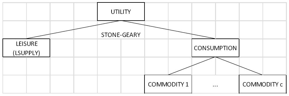
For private consumption we assume that there is a single representative household that allocates its disposable income across the various commodities according to a Stone-Geary utility function. This functional form has the advantage of allowing for commodity-specific income elasticities. The government collects taxes, makes and receives transfers, and purchases commodities. The behavior of the government receipts and spending depends on the selected macroeconomic closure rule (see below).
Argentina is modeled as a small open economy that takes the prices of exports and imports as givens. By following the Armington assumption (Armington, 1969; de Melo & Robinson, 1989), products are differentiated according to their country of origin (domestic versus imports) and destination (domestic versus exports). As usual, a sectoral CES and a sectoral CET are used for consumption and production, respectively.
The labor market is the main channel of interaction between the CGE model and the microsimulation model. We build a model with endogenous labor supply and unemployment. The labor market is segmented between rural (agricultural) and urban (non-agricultural) activities9, with perfect mobility within a given segment but imperfect mobility between segments. Labor moves between rural and urban activities according to a CET function. In each segment, we assume the existence of a downward-rigid real wage for each type of labor. The minimum real wage for each skill level varies with the following determinants: the unemployment rate as in a wage curve, real living standards captured by household consumption per capita, average real factor returns (price of value-added), and the consumer price index.10 The labor-leisure choice is modeled according to a Stone-Geary utility function as in de Melo and Tarr (1992). We assume a minimal level of leisure in the utility function along with a minimal level consumption of each good. Figure 2 shows the representative household decision tree.

The consumption side.
In order to better capture the tax system of Argentina, our model incorporates a value-added tax with rebates for intermediate input and investment purchases as in Go et al. (2005). With this treatment, there is no cascading effect on prices of taxes on intermediate goods. We assume the VAT is administered using the “invoice method”. All transactions are taxed at a fixed proportional rate regardless of whether they are final or intermediate transactions. Firms can deduct taxes paid on intermediate inputs and that tax amount is reported on the invoices for intermediates. Import sales are subject to a VAT, while export sales are not.
As is the usual case (Robinson, 2006), we need to specify the three macroeconomic balances that are usually present in a CGE model: i) external balance, ii) savings-investment, and iii) government budget. The model allows for alternative closure rules for these balances. In the following section we explain the macroeconomic closure rules used for each simulation.
The model is formulated as a static model that is solved sequentially over time. In each period the following variables are updated: physical sectoral capital stocks, population, labor force disaggregated by skill level, LES (linear expenditure system) minimal consumption, and technological change.
The process of physical capital accumulation is endogenous with previous-period investment generating new capital stock for the subsequent period. The allocation of new capital across sectors is influenced by two factors: i) each sector’s initial share of aggregate capital income, and ii) sectoral profit-rate differentials from the previous period. Sectors with above (below) average capital returns will receive a larger (smaller) share of total investment than their share in capital income. A similar approach is followed by Dervis et al. (1982) and more recently by Thurlow (2004) in his extension of the IFPRI Standard Model.
Population growth is exogenously imposed on the model based on separately calculated growth projections – the average annual total population growth rate is one percent. We make a distinction between total population and the labor force. Thus, based on past trends from population census data, we assume an exogenous growth path for the population in labor force age with skilled population growing faster than unskilled population11; the initial skill composition of the labor force is 53 percent unskilled, 32 percent semi-skilled, and 15 percent skilled. The transfers between different institutions are assumed to change at the same (exogenous) base GDP growth rate.
Micro simulation
The microsimulation model generates a counterfactual household income distribution for each time period of the simulation. Let Yt be the household income distribution in year t, which can be written as a function F of the labor income (
We can simulate the income distribution in a given year t by changing the arguments in equation (1).
As explained, the EPH corresponding to the year 2005 was used as our main data for the microsimulation model. The microsimulation model considers the following eight effects that are simulated cumulatively; that is, the current effect is simulated on top of the previous effect.12
Population growth
The first effect consists of individual re-weighting in order to reflect the population growth over time. First, we change the individual weights based on population forecasts by age brackets and gender from INDEC; the new weights are computed taking into account that individuals in the same household should have the same weights. Second, we rescale all individual weights in order to replicate total population growth from INDEC; this last adjustment is implemented because the age and gender structure in the household survey are not necessarily identical to that in the population projections. Additionally, this reweighting of individuals and households also takes into account exogenous changes in the educational structure of the workforce.
Participation rate
In this step, the participation rate (i.e., the size of the labor supply) of each labor category – identified based on skill level – is changed according to the CGE results. Recall that the CGE model endogenizes the labor-leisure choice. The participation rate is defined as the ratio between the labor force and the total population in each labor category. Individuals who change their labor status are randomly selected. The counterfactual labor income of the newly active individuals is assigned after the unemployment rate and the sectoral structure of employment effects are introduced.
Unemployment rate
This effect moves individuals between employment and unemployment such that the change in the unemployment rate from the CGE model is replicated. The individuals who change their labor status are randomly selected. The counterfactual employment level (e) results from the combination of the participation rate (a) and the unemployment rate (u), according to the formula e=(1-u)a. The counterfactual labor income of those individuals who move from unemployment to employment is assigned in the next step of the microsimulation model, once they are allocated to a counterfactual sector of employment.
Sectoral structure of employment
This effect replicates the change in the sectoral structure of employment that results from the CGE model. In each period, depending on the previous effects, employed individuals can be classified into three groups: (1) those who were working in the previous period; (2) those who moved from unemployment to employment; and (3) those who moved from inactivity to being employed. The new workers are the first to be assigned to the expanding sectors. Within each group, the individuals who change their sector of employment are randomly selected. For those individuals who change their sector of employment a counterfactual labor income is estimated using the coefficients from a Mincerian wage equation, plus a random shock.13 Finally, for those individuals who move from employment to inactivity or unemployment a counterfactual labor income of zero is assigned.
Relative wages
First, we modify individual wages according to the results generated by the CGE model for each labor category. We then rescale individual wages so as to keep the average wage constant.
Average wage
We simply multiply all individual wages that result from the previous effect by the same scalar to reflect the change in the average wage generated by the CGE model.
Non-labor factor income
We increase the non-labor factor income in t-1 by applying the change in the rate of return to non-labor factors (capital, land, natural resources) from the CGE model.14
Poverty line
The value of the extreme (food) poverty line is determined endogenously within the CGE model as in Decaluwé et al. (1999). This is possible because all the commodity prices are endogenous in the CGE model. The counterfactual value for the moderate poverty line is computed by applying the inverse of the Engel coefficient to the value of the extreme poverty line.
This sequence for introducing changes in the selected labor market parameters is similar to that of Vos et al. (2002). However, our approach is different in that we use econometric estimations to assign counterfactual wages to those individuals who change their labor market situation in a counterfactual scenario, with the last step involving a change in the poverty line that reflects the price movement of different goods. The microsimulation model is solved several times15, due to the use of random numbers at different steps in the process. This allows us to construct confidence intervals for the poverty and inequality results.
At every step of the microsimulation a counterfactual labor income for each individual in the workforce is generated. This new labor income distribution is used to compute a counterfactual household income. Additionally, at the last step a new poverty line is also computed. We then calculate several standard inequality and poverty indicators such as the Gini coefficient and the poverty headcount ratio.
Macro-Micro interaction
The two models are used in a sequential top-down fashion. The (macro) CGE model communicates with the microsimulation model by generating a vector of prices, (urban) wages, and aggregate employment variables such as labor supply and (urban) unemployment. The functioning of the labor market plays an important role in this regard. The dynamic nature of our macro-micro model allows us to track the effect of economic policies and external shocks on poverty and inequality on a period by period basis.
Only the percentage deviations from the baseline are transmitted from the CGE model to the microsimulation model. Consequently, we do not assure complete consistency (i.e., that absolute aggregate magnitudes are equal) between the data sets used at the two modeling stages (see Bourguignon et al., 2008).
3. Simulations
3.1 Scenarios
The scenarios that we consider can be divided into two groups (see Table 4). On the one hand, there are simulations of the elimination of export duties introduced during the 2001–2002 crisis. On the other hand, there are simulations of changes in world food and oil prices. In both cases, special emphasis is placed on their effects on the fiscal situation. As was mentioned, both short-and long-run effects are analyzed.
CGE-microsimulations scenarios.
| Name | Description |
|---|---|
| base | Business as usual scenario |
| Policy shockx | |
| Etax-gsav | 20% yearly cut in export tax with government savings as the equilibrating variable |
| Etax-gcon | 20% yearly cut in export tax with government consumption as the equilibrating variable |
| Etax-dtax | 20% yearly cut in export tax with direct tax rate as the equilibrating varialbe |
| External shockx | |
| Wprice-food | 25% decrease in world food prices in 2008 |
| Wprice-oil | 25% decrease in world oil prices in 2008 |
The first group of scenarios is motivated by the debate over export duties in Argentina, particularly regarding their level. The second group of scenarios is related to the strong increase in food prices seen during the second half of the 2000s. As Argentina is an important food exporter, there is a need to assess the effects of a reduction in world food prices. In addition, as it was mentioned above, the highest export tax rates are applied on products whose international price has shown volatile behavior recently.
In the scenarios of export tax reduction, three financing alternatives are employed to balance the government account: (i) financing through debt (that is, government savings are flexible); (ii) public spending is the adjustment variable (that is, it decreases in response to a fall in tax revenues); and (iii) the direct tax rate is endogenously adjusted to keep government savings constant at the baseline level (i.e., at around 5% of GDP).
In the export tax scenarios we simulate a 20 percent yearly reduction starting in year 2008 (cumulating to a 2/3 reduction by 2013) of the export tax that was introduced during the 2001/02 economic crisis. The relevance of this tax change had already been discussed by many observers (see Llach and Harriague, 2005). In turn, the reduction in world food and oil prices is simulated as a fall both in export and import prices.
3.2 Results
We show results in terms of aggregate welfare, sectoral output, sectoral trade, unemployment, terms of trade, prices of commodities, and wages from the CGE model. Using the microsimulation model we compute results in terms of inequality and poverty. The differences between the counterfactual scenarios and the baseline scenario are interpreted as the economy-wide impact of the simulated shocks.
Baseline scenario
The first (base) scenario is a business-as-usual scenario. Accordingly, this scenario reflects the economy’s evolution in the absence of shocks. In order to produce a baseline scenario, total factor productivity is adjusted to generate an annual growth rate for real GDP at factor cost that replicates the behavior of the Argentine economy for the period 2005–2008 and decreases thereafter, reaching an annual growth rate of 3.5 percent in year 2010.16
As said before, the model has three balances at the macro level. The absorption shares of government spending, total investment, and household consumption are kept constant in order to produce a “balanced” closure. This closure mimics Argentina’s past experience with simultaneous adjustments in the three components of absorption. The value of private savings is determined endogenously to maintain the balance between investment and total savings; the ratio between investment and absorption follows an exogenous path.17 The real exchange rate varies in order to equilibrate the total inflows and outflows of foreign exchange, keeping foreign savings fixed as a share of GDP. The transfers from the rest of the world to the domestic institutions are set to grow exogenously at the same rate as real GDP, expressed in foreign currency. The transfers between the government and households grow exogenously at the same rate as real GDP. The model numeraire is the consumer price index. Finally, all tax rates are fixed over time. The model also considers the quantitative restrictions on exports of agri-food products that were introduced in 2006.
The poverty rate in the baseline scenario diminishes from 33.8 percent, observed in 2005, to around 25.7 percent in 2015, mainly as a consequence of an increase in the average wage rate (see Table 9). The implicit growth elasticity of poverty for the period 2005–2015 is approximately 0.48. The Gini coefficient does not show any significant change throughout the whole simulation period.
Counterfactual scenarios
The method used to balance government accounts vary across the simulations. Specifically, we
consider three closure rules in the policy-induced simulations (see above), and assume that government savings are flexible in the external shocks simulations. Real investment is endogenous and driven by total savings; thus, the model captures growth effects that result from changes in investment. Foreign savings are fixed through an endogenous real exchange rate.
Policy shocks
In aggregate terms, the reduction in export taxes has different effects in the short- and long-run, when the government budget is balanced either through direct taxes (see etax-dtax scenario) or government consumption (see etax-gcon scenario) (see Table 5 and Table A.2 in the Appendix). In the short run, a fall in GDP is observed, which can be accounted for by several factors. When the export tax is eliminated, the sectors with the highest tax rates expand their production level (see below). As was shown, these sectors are, in relation to the rest of the economy, relatively capital-intensive (particularly in land). Consequently, when expanded, they cannot absorb all the labor – specifically semi-skilled and skilled labor – that is expelled by the sectors that are contracting, and consequently urban unemployment increases at the same time that rural unemployment decreases (see Table 6); at the national level however, total unemployment increases.18 Additionally, a fall in the national labor supply is observed, particularly when government savings and public consumption are used to balance the government budget. The decrease in the participation rate combined with the increase in the urban unemployment rate impact negatively on poverty (see Table 9) On the other hand, the increase in the returns to the land, combined with the reduction in the rural unemployment rate, reduce rural poverty which, according to the scarce available evidence, is higher than urban poverty.19 Overall, national poverty increases since the number of households escaping poverty in the rural areas does not compensate for the number of households entering poverty in the urban areas; recall that (1) the share of urban areas in Argentina is 87.1 percent, and (2) the baseline unemployment rate is higher in urban areas (see Table 6).
In the long run, the reallocation of resources generates an increase in the returns to capital, land and natural resources, which drives higher private savings, even with a higher direct tax in the etax-dtax scenario. As a result, investment is higher than in the baseline scenario, driving an increased in the capital stock that results in a growth rate that is slightly higher than in the baseline scenario (see Table 5). However, when government financing is through debt, there is a fall in investment that reduces the economy’s growth rate throughout the simulation period. That is to say, the need for public financing reduces the savings available for investment.
Real macro indicators by simulation (annual growth rate 2007–2015).
| indicator | Base (LCU$) | Base (chg%) | Policy shocks | External shocks | |||
|---|---|---|---|---|---|---|---|
| Etax-gsav | Etax-gcon | Etax-dtax | Wp-food | Wp-oil | |||
| Absorption | 5,033 | 3.9 | 3.7 | 4.0 | 4.0 | 3.2 | 3.7 |
| Household consumption | 3,263 | 3.8 | 3.9 | 4.1 | 3.9 | 3.4 | 3.8 |
| Government consumption | 657 | 4.1 | 4.1 | 2.9 | 4.1 | 4.1 | 4.1 |
| Fixed investment | 1,114 | 3.9 | 3.1 | 4.4 | 4.2 | 2.2 | 3.4 |
| Exports | 1,365 | 3.8 | 4.0 | 4.4 | 4.3 | 3.7 | 3.8 |
| Imports | −1,041 | 3.8 | 4.1 | 4.6 | 4.5 | 2.7 | 3.5 |
| GDP market price | 5,358 | 3.9 | 3.7 | 4.0 | 4.0 | 3.4 | 3.8 |
| GDP factor cost | 4,434 | 3.9 | 3.7 | 4.0 | 4.0 | 3.6 | 3.8 |
| Real exchange rate | 1 | 0.1 | −0.4 | −0.4 | −0.4 | 0.9 | 0.3 |
-
Source: Author’s estimates.
Unemployment rate by labor type in base year and final year by simulation (%).
| 2015 (final year) | |||||||
|---|---|---|---|---|---|---|---|
| Labor category | 2005 | base | Etax-gsav | Etax-gcon | Etax-dtax | Wp-food | Wp-oil |
| Urban | |||||||
| – Unskilled labor | 19.1 | 13.8 | 14.2 | 13.9 | 14.0 | 14.2 | 13.8 |
| – Semi-skilled labor | 14.6 | 10.6 | 11.0 | 10.7 | 10.8 | 11.0 | 10.6 |
| – Skilled labor | 5.5 | 2.8 | 3.2 | 2.9 | 3.0 | 3.2 | 2.8 |
| – Total | 15.7 | 10.9 | 11.3 | 11.0 | 11.1 | 11.3 | 10.9 |
| Rural | |||||||
| – Unskilled labor | 13.1 | 7.4 | 7.5 | 7.0 | 7.2 | 10.1 | 7.4 |
| – Semi-skilled labor | 10.0 | 6.4 | 6.5 | 6.0 | 6.2 | 9.1 | 6.4 |
| – Skilled labor | 3.8 | 2.5 | 2.5 | 2.5 | 2.5 | 5.0 | 2.5 |
| – Total | 10.7 | 6.2 | 6.3 | 5.9 | 6.1 | 8.9 | 6.2 |
| National | |||||||
| – Unskilled labor | 18.5 | 13.2 | 13.6 | 13.3 | 13.3 | 13.9 | 13.2 |
| – Semi-skilled labor | 14.4 | 10.4 | 10.8 | 10.5 | 10.6 | 10.9 | 10.4 |
| – Skilled labor | 5.4 | 2.8 | 3.2 | 2.9 | 2.9 | 3.3 | 2.8 |
| – Total | 15.3 | 10.5 | 10.9 | 10.6 | 10.7 | 11.1 | 10.5 |
-
Source: Author’s estimates.
The loss of tax revenues due to the elimination of export duties is not automatically compensated by an increase in revenues from other tax instruments (see Table 7). As a consequence, it either generates: (1) a reduction in public savings (etax-gsav scenario) by 1.7 percentage points of GDP by 2015, or (2) a reduction in public consumption (etax-gcon scenario) by 1.3 percentage points of GDP. In the first case, a crowding-out effect that reduces investment takes place. As a consequence, growth declines; in the 2007–2015 period, the annual growth rate falls from 3.9 percent in the base scenario to 3.7 percent in the etax-gsav scenario (see Table 5). However, when the elimination of export duties is compensated with a reduction in government consumption, the average annual growth rate for 2007–2015 slightly increases to reach 4 percent.20
Fiscal indicators.
| 2015 (final year) | |||||||
|---|---|---|---|---|---|---|---|
| Labor category | 2005 | base | Etax-gsav | Etax-gcon | Etax-dtax | Wp-food | Wp-oil |
| Gov consumption (share GDP) | 12.3 | 12.3 | 12.4 | 11.0 | 12.2 | 12.9 | 12.4 |
| Gov savings (share GDP) | 4.9 | 4.9 | 3.2 | 4.9 | 4.9 | 3.5 | 4.3 |
| Tax revenue(share GDP) | 28.0 | 28.0 | 26.6 | 26.7 | 27.9 | 27.8 | 27.8 |
| – Export tax | 2.3 | 2.1 | 0.4 | 0.4 | 0.4 | 1.7 | 2.0 |
| – Tariffs | 0.7 | 0.8 | 0.7 | 0.8 | 0.8 | 0.8 | 0.8 |
| – Value added tax | 6.9 | 6.9 | 6.9 | 6.9 | 6.9 | 6.9 | 6.8 |
| – Other indirect taxes | 7.3 | 7.4 | 7.6 | 7.6 | 7.6 | 7.5 | 7.2 |
| – Direct taxes | 10.8 | 10.9 | 11.0 | 11.0 | 12.2 | 10.9 | 10.9 |
-
Source: Author’s estimates.
As expected, export volumes increase in all export tax elimination scenarios; on average, export prices are around 4.2 percent higher than in the baseline in 2015. As a result, an appreciation of the real exchange rate takes place in order to balance the current account (see Table 5).
As producers reorient toward export markets, there is an increase in the domestic prices. This increase in domestic food prices has a negative effect on poverty by increasing the poverty line (again, see Table 9). At the same time, an increase in domestic prices of intermediate inputs raises costs for domestic processing industries.
As expected, after the elimination of export duties, the sectors that expand most are those that, at the beginning, faced the highest export tax rates. At the same time, the effect of rising primary exports is an appreciation of the real exchange rate, which undermines the competitiveness of other agricultural and manufacturing exports (see Table 8). A significant change in the sectoral composition of Argentina’s economic structure can be observed. In particular, both production and exports turn towards primary products. At the same time, imports of manufactures increase, replacing domestic production. Argentina’s productive structure is thus modified with primary products such as cereals, oil seeds, oil, and vegetable oils and fats gaining importance.
Sectoral results by simulation (annual growth rate 2007–2015).
| Indicator | Base (LCU$) | Base (chg %) | Policy shocks | External shocks | |||
|---|---|---|---|---|---|---|---|
| Etax-gsav | Etax-gcon | Etax-dtax | Wp-food | Wp-oil | |||
| GDP primary | 596 | 2.9 | 3.1 | 3.3 | 3.3 | 1.9 | 2.6 |
| GDP non-primary | 3,837 | 4.1 | 3.8 | 4.1 | 4.1 | 3.8 | 4.0 |
| Exports primary | 320 | 2.1 | 4.5 | 4.7 | 4.8 | 1.2 | 2.1 |
| Imports primary | 47 | 4.3 | 6.2 | 6.6 | 6.5 | 3.4 | 3.9 |
| Exports non-primary | 1,045 | 4.2 | 3.9 | 4.3 | 4.2 | 4.3 | 4.2 |
| Imports non-primary | 994 | 3.7 | 4.0 | 4.5 | 4.4 | 2.6 | 3.5 |
-
Source: Author’s estimates.
Microsimulation results – changes in poverty (*) Official moderate poverty rate (change in percentage points).
| Policy shocks | External shocks | ||||
|---|---|---|---|---|---|
| Microsimulation effect | Etax-gsav | Etax-gcon | Etax-dtax | Wp-food | Wp-oil |
| Pop | 0.05 | 0.00 | 0.01 | 0.06 | 0.00 |
| Pop + act | −0.05 | 0.00 | −0.02 | −0.03 | 0.01 |
| Pop+ act + uerat | 0.03 | 0.06 | −0.01 | 0.06 | 0.01 |
| Pop + act + uerat + sec | −0.01 | −0.03 | 0.07 | −0.04 | 0.00 |
| Pop + act + uerat + sec + w1 | 0.04 | −0.05 | 0.00 | 0.05 | −0.08 |
| Pop + act + uerat + sec + w1 + w2 | 0.59 | 0.10 | 0.20 | 0.68 | 0.08 |
| Pop + act + uerat + sec + w1 + w2 + cap | 0.00 | −0.02 | −0.01 | 0.04 | 0.00 |
| Pop + act + uerat + sec + w1 + w2 + cap + pl | 1.16 | 1.62 | 1.42 | −3.91 | 0.20 |
| TOTAL | 1.81 | 1.68 | 1.66 | −3.09 | 0.23 |
-
Source: Author’s estimates.
-
(*)
other poverty indicators are available from the authors upon request.
-
Notes: pop = population; act = participation rate; uerat = unemployment rate; sec = sector structure employment; w1 = relative wages; w2 = average wage; cap = non-labor incomes; pl=poverty line.
The production of oil seeds aimed at the domestic market increases considerably since it constitutes the most important individual intermediate input in the production of vegetable oils and fats, which is the main Argentine export product.
Export tax cuts increase the price of the intermediate inputs used by the sectors that process raw products such as Dairy products, Beverages and tobacco, among others, due to the fact that export tax rates were initially highest for primary products. This effect also contributes to the expansion of primary sectors vis-à-vis manufacturing sectors.
External shocks
In this section the impact of a decline in world food and oil prices is analyzed. In this case, it is assumed that the adjustment variable for the government is government savings.
The fiscal situation deteriorates, mainly as a consequence of a reduction in export tax revenues. The government surplus as a share of GDP is 1.4 percentage points lower in 2015 in the food price reduction scenario (wp-food) than in the baseline scenario. This generates a crowding-out effect of investment, which reduces GDP growth and increases unemployment, mainly rural unemployment (see Tables 5-7).
When world food prices fall, there is a negative effect both in the short- and long- run (see Table A.2). As was previously described, Argentina is a net agri-food exporter. Consequently, this shock constitutes a worsening in Argentina’s terms of trade. Economic indicators as a whole worsen. The growth rate of the GDP at factor cost for the 2007–2015 period falls by 0.3 percentage points (see scenario wp-food). The decrease in the growth rate is higher for primary than for non-primary activities (see Table 8). Moreover, the national unemployment rate increases by 5.4 percent in 2015 with respect to the baseline scenario, mainly due to a strong increase in the rural unemployment rate.21
On the other hand, domestic food prices decrease, which has a positive impact on poverty. In the end, poverty declines due to the poverty line effect but increases due to the unemployment and the average wage effects (see Table 9). Poverty increases more in rural areas due to a larger decrease in rural labor and non-labor income.
The decrease in the oil price also reduces the GDP growth rate – about 0.1 percent yearly, although the impact is lower than in the food price scenario. This is expected since oil is a less relevant product in the Argentinean economy than agri-food products. As before, fiscal revenues are reduced, decreasing government savings. In turn, this generates a crowding out effect of investment.
4. Concluding remarks
In this paper we conducted a quantitative general equilibrium analysis on a sensitive economic and political debate (i.e., export taxes) in Argentina.
In order to provide an empirical assessment, we implemented a (top-down) CGE-microsimulation framework. This study analyzed the economy-wide impact of (1) a gradual elimination of the export tax that was introduced after the 2001/2002 economic crisis, and (2) a decrease in the world price of Argentina’s main export products: food and oil. We found that the elimination of the export tax would have different long run effects depending on the fiscal instrument that is used by the government to compensate for the loss in tax revenue. On the one hand, when the government budget is balanced by decreased government savings, the average annual growth rate for 2008–2015 is lower than in the baseline scenario. On the other hand, when the government budget is balanced by an increased direct tax rate, there is a long- run positive effect on growth. In any case, the employment level is lower (i.e., participation rate decreases at the same time that unemployment rate increases) and the price of food items is higher.22 Therefore, the poverty headcount ratio increases.
As expected, a reduction in the world food prices (i.e., a worsening in Argentina’s terms of trade) would impact negatively on the country’s GDP growth rate and poverty, particularly in the rural areas.
Footnotes
1.
Tariff escalation refers to the practice in some high-income countries of charging high tariffs on processed goods and lower or no tariffs on primary products, thus granting a higher effective rate of protection to value-added in the importing country. Consequently, tariff escalation in developed countries discourages diversification of production and increases their reliance on unprocessed goods.
2.
Indeed, one of the justifications for export taxes in the literature is to “decouple” domestic prices from world prices (Devarajan et al., 1996; Piermartini, 2004; Bouët and Laborde, 2012).
3.
In December 2015, export tax rates were decreased, and even eliminated for some products such as wheat and meat.
4.
In Mercado (2003) only two “institutional” CGE models are surveyed, and – to the best of our knowledge – the number has not increased since.
5.
On the other hand, there are some applications of the CGE methodology to Argentina; see, for example, Chisari et al. (1999) and Wang et al. (1995).
6.
Notice that we found that the CGE results were sensible to the sectoral disaggregation in the SAM.
7.
The microdata of the EPH is available for the Greater Buenos Aires (GBA) area beginning 1974, while the rest of the urban areas have been added during the last three decades.
8.
However, whenever possible, we complement our analysis with the scarce available information on rural poverty in Argentina.
9.
The activities classified as rural are Cereals, Vegetables and fruits, Oil seeds, Other crops, and Livestock, milk and wool.
10.
Our formulation for the downward rigid real wage can be derived from the efficiency wage literature as described, among others, in Boeters and Savard (2013).
11.
We refer to the CGE model variable named MAXHOUR; see the model mathematical statement In the one-line Appendix B.
12.
The microsimulation effects are also simulated individually; this alternative set of results is available from the authors upon request. Note that a certain sequence must be assumed regarding how different dimensions of aggregate labor market changes (e.g., changes in unemployment rates). Consequently, as with other microsimulation approaches, a problem of path dependence can be present. However, we can justify the logic of the followed sequence on the basis of plausible labor market behavior and as long as the size of the simulated shifts is not very large (see Vos and Sanchez, 2010).
13.
The explanatory variables included in the equation are experience and experience squared, dummies per sector, regional dummies, and marital status. The individuals included in the regression are those who were employed in t-1 and still in t.
14.
However, notice that the underreporting of non-labor factor income is very important in the Argentinean household survey (Gasparini, 1999). See also Deaton (1997).
15.
Specifically, we considered 100 draws. However, after 30 draws results barely change.
16.
The 3.5% growth rate was obtained using data on factor endowments for the period 1990–2001 to compute potential GDP for Argentina.
17.
In order to generate savings that equal the cost of investment, the savings rate of the representative household is endogenously adjusted.
18.
When the model is run with full employment and with no leisure-consumption choice, a fall in wages is obtained.
19.
In a recent study, Guardia and Tornarolli (2009) survey all the (scarce) available sources of information regarding rural poverty in Argentina; they found that rural poverty is significantly higher than urban poverty, but both follow a similar evolution in time.
20.
However, notice that we are not considering the negative growth effect that reduced public spending in infrastructure may have.
21.
Notice that we are not considering the negative growth effect that reduced public spending in infrastructure may have.
22.
As shown in Section 3, the employment level is lower than in the baseline scenario due to the change in the sectoral composition of Argentina’s productive structure.
Appendix A: additional tables
Export tax rates and tariffs rates (%).
| Export tax | Tariffs | |
|---|---|---|
| Sector | (i) | (ii) |
| Primary | ||
| Cereals | 14.5 | 2.4 |
| Vegetables and fruits | 7.3 | 3.6 |
| Oil seeds | 20.0 | 2.3 |
| Other crops | 7.3 | 2.8 |
| Livestock, milk and wool | 10.9 | 1.9 |
| Other non agr primary | 3.6 | 1.5 |
| Mining | 3.6 | 0.4 |
| oil | 32.7 | |
| Processed food | ||
| Meat | 10.9 | 4.0 |
| Other proc food | 3.6 | 4.8 |
| Vegetable oils and fats | 17.4 | 3.8 |
| Dairy products | 3.6 | 5.6 |
| Sugar | 3.6 | 6.7 |
| Beverages and tobacco | 3.6 | 7.0 |
| Other manufactures | ||
| Textiles and apparel | 3.6 | 6.4 |
| Other manufacturing | 3.6 | 5.2 |
| Petroleum refinery | 3.6 | 0.1 |
| Chemical products | 3.6 | 2.8 |
| Mineral products | 3.6 | 4.2 |
| Metal products | 3.6 | 4.2 |
| Machinery and equipment | 3.6 | 4.7 |
| vehicules | 3.6 | 9.0 |
-
Source: Argentina SAM 2005.
Real macro indicators by simulation and year (growth rate).
| Indicator | Scenario | 2005 | 2006 | 2007 | 2008 | 2009 | 2010 | 2011 | 2012 | 2013 | 2014 | 2015 |
|---|---|---|---|---|---|---|---|---|---|---|---|---|
| Absorption | base | 5,033 | 8.0 | 7.9 | 6.5 | 4.0 | 3.5 | 3.5 | 3.5 | 3.5 | 3.5 | 3.4 |
| Household consumption | base | 3,263 | 8.0 | 8.0 | 6.4 | 3.9 | 3.4 | 3.4 | 3.4 | 3.4 | 3.4 | 3.4 |
| Government consumption | base | 657 | 8.1 | 7.9 | 6.9 | 4.2 | 3.7 | 3.7 | 3.6 | 3.6 | 3.6 | 3.6 |
| Fixed investment | base | 1,114 | 7.9 | 7.8 | 6.6 | 4.0 | 3.5 | 3.5 | 3.5 | 3.5 | 3.5 | 3.5 |
| Exports | base | 1,365 | 7.8 | 7.7 | 6.5 | 3.8 | 3.3 | 3.3 | 3.3 | 3.3 | 3.3 | 3.3 |
| Imports | base | −1,041 | 7.8 | 7.7 | 6.5 | 3.8 | 3.3 | 3.3 | 3.3 | 3.3 | 3.3 | 3.3 |
| GDP market price | base | 5,358 | 8.0 | 7.9 | 6.5 | 4.0 | 3.5 | 3.5 | 3.5 | 3.4 | 3.4 | 3.4 |
| GDP factor cost | base | 4,434 | 8.0 | 8.0 | 6.5 | 4.0 | 3.5 | 3.5 | 3.5 | 3.5 | 3.5 | 3.5 |
| Real exchange rate | base | 1 | 0.2 | 0.5 | −0.3 | 0.1 | 0.1 | 0.2 | 0.2 | 0.2 | 0.2 | 0.1 |
| Absorption | etax-gsav | 5,033 | 8.0 | 7.9 | 6.6 | 3.9 | 3.4 | 3.3 | 3.2 | 3.2 | 3.2 | 3.2 |
| Household consumption | etax-gsav | 3,263 | 8.0 | 8.0 | 6.8 | 4.2 | 3.6 | 3.5 | 3.4 | 3.3 | 3.3 | 3.2 |
| Government consumption | etax-gsav | 657 | 8.1 | 7.9 | 6.9 | 4.2 | 3.7 | 3.7 | 3.6 | 3.6 | 3.6 | 3.6 |
| Fixed investment | etax-gsav | 1,114 | 7.9 | 7.8 | 5.8 | 3.1 | 2.6 | 2.6 | 2.6 | 2.6 | 2.6 | 2.7 |
| Exports | etax-gsav | 1,365 | 7.8 | 7.7 | 7.2 | 4.3 | 3.7 | 3.6 | 3.5 | 3.4 | 3.3 | 3.3 |
| Imports | etax-gsav | −1,041 | 7.8 | 7.7 | 7.4 | 4.5 | 3.8 | 3.7 | 3.5 | 3.4 | 3.3 | 3.3 |
| GDP market price | etax-gsav | 5,358 | 8.0 | 7.9 | 6.6 | 3.9 | 3.4 | 3.3 | 3.3 | 3.2 | 3.2 | 3.2 |
| GDP factor cost | etax-gsav | 4,434 | 8.0 | 8.0 | 6.4 | 3.9 | 3.3 | 3.3 | 3.3 | 3.2 | 3.2 | 3.2 |
| Real exchange rate | etax-gsav | 1 | 0.2 | 0.5 | −1.1 | −0.6 | −0.5 | −0.4 | −0.3 | −0.3 | −0.2 | −0.2 |
| Absorption | etax-gcon | 5,033 | 8.0 | 7.9 | 6.6 | 4.1 | 3.6 | 3.6 | 3.6 | 3.6 | 3.6 | 3.6 |
| Household consumption | etax-gcon | 3,263 | 8.0 | 8.0 | 6.8 | 4.3 | 3.8 | 3.7 | 3.7 | 3.6 | 3.6 | 3.6 |
| Government consumption | etax-gcon | 657 | 8.1 | 7.9 | 4.4 | 2.1 | 2.0 | 2.3 | 2.7 | 2.9 | 3.1 | 3.3 |
| Fixed investment | etax-gcon | 1,114 | 7.9 | 7.8 | 7.3 | 4.6 | 4.0 | 4.0 | 3.9 | 3.8 | 3.8 | 3.8 |
| Exports | etax-gcon | 1,365 | 7.8 | 7.7 | 7.4 | 4.6 | 4.0 | 4.0 | 3.9 | 3.8 | 3.8 | 3.7 |
| Imports | etax-gcon | −1,041 | 7.8 | 7.7 | 7.6 | 4.8 | 4.2 | 4.1 | 4.0 | 4.0 | 3.9 | 3.8 |
| GDP market price | etax-gcon | 5,358 | 8.0 | 7.9 | 6.6 | 4.1 | 3.6 | 3.6 | 3.6 | 3.6 | 3.6 | 3.6 |
| GDP factor cost | etax-gcon | 4,434 | 8.0 | 8.0 | 6.5 | 4.0 | 3.6 | 3.6 | 3.6 | 3.6 | 3.6 | 3.6 |
| Real exchange rate | etax-gcon | 1 | 0.2 | 0.5 | −1.0 | −0.5 | −0.5 | −0.4 | −0.3 | −0.3 | −0.2 | −0.2 |
| Absorption | etax-dtax | 5,033 | 8.0 | 7.9 | 6.6 | 4.1 | 3.6 | 3.6 | 3.5 | 3.5 | 3.5 | 3.5 |
| Household consumption | etax-dtax | 3,263 | 8.0 | 8.0 | 6.4 | 4.0 | 3.5 | 3.5 | 3.5 | 3.5 | 3.5 | 3.5 |
| Government consumption | etax-dtax | 657 | 8.1 | 7.9 | 6.9 | 4.2 | 3.7 | 3.7 | 3.6 | 3.6 | 3.6 | 3.6 |
| Fixed investment | etax-dtax | 1,114 | 7.9 | 7.8 | 7.0 | 4.3 | 3.8 | 3.7 | 3.7 | 3.7 | 3.7 | 3.6 |
| Exports | etax-dtax | 1,365 | 7.8 | 7.7 | 7.3 | 4.5 | 3.9 | 3.9 | 3.8 | 3.7 | 3.7 | 3.6 |
| Imports | etax-dtax | −1,041 | 7.8 | 7.7 | 7.5 | 4.7 | 4.1 | 4.0 | 3.9 | 3.9 | 3.8 | 3.7 |
| GDP market price | etax-dtax | 5,358 | 8.0 | 7.9 | 6.6 | 4.1 | 3.5 | 3.5 | 3.5 | 3.5 | 3.5 | 3.5 |
| GDP factor cost | etax-dtax | 4,434 | 8.0 | 8.0 | 6.5 | 4.0 | 3.5 | 3.5 | 3.5 | 3.5 | 3.5 | 3.5 |
| Real exchange rate | etax-dtax | 1 | 0.2 | 0.5 | −1.1 | −0.6 | −0.5 | −0.4 | −0.3 | −0.3 | −0.2 | −0.2 |
| Absorption | wp-food | 5,033 | 8.0 | 7.9 | 4.1 | 3.5 | 3.0 | 3.0 | 3.0 | 3.0 | 3.0 | 3.1 |
| Household consumption | wp-food | 3,263 | 8.0 | 8.0 | 5.2 | 3.5 | 3.0 | 3.1 | 3.1 | 3.1 | 3.1 | 3.1 |
| Government consumption | wp-food | 657 | 8.1 | 7.9 | 6.9 | 4.2 | 3.7 | 3.7 | 3.6 | 3.6 | 3.6 | 3.6 |
| Fixed investment | wp-food | 1,114 | 7.9 | 7.8 | −0.6 | 2.9 | 2.4 | 2.5 | 2.5 | 2.5 | 2.5 | 2.6 |
| Exports | wp-food | 1,365 | 7.8 | 7.7 | 10.0 | 3.1 | 2.6 | 2.7 | 2.7 | 2.7 | 2.8 | 2.8 |
| Imports | wp-food | −1,041 | 7.8 | 7.7 | 1.0 | 3.3 | 2.8 | 2.8 | 2.8 | 2.9 | 2.9 | 2.9 |
| GDP market price | wp-food | 5,358 | 8.0 | 7.9 | 6.2 | 3.4 | 2.9 | 3.0 | 3.0 | 3.0 | 3.0 | 3.0 |
| GDP factor cost | wp-food | 4,434 | 8.0 | 8.0 | 6.8 | 3.5 | 3.0 | 3.0 | 3.0 | 3.1 | 3.1 | 3.1 |
| Real exchange rate | wp-food | 1 | 0.2 | 0.5 | 7.3 | 0.1 | 0.1 | 0.1 | 0.1 | 0.1 | 0.1 | 0.1 |
| Absorption | wp-oil | 5,033 | 8.0 | 7.9 | 5.9 | 3.8 | 3.3 | 3.3 | 3.3 | 3.3 | 3.3 | 3.3 |
| Household consumption | wp-oil | 3,263 | 8.0 | 8.0 | 6.4 | 3.8 | 3.3 | 3.3 | 3.3 | 3.3 | 3.3 | 3.3 |
| Government consumption | wp-oil | 657 | 8.1 | 7.9 | 6.9 | 4.2 | 3.7 | 3.7 | 3.6 | 3.6 | 3.6 | 3.6 |
| Fixed investment | wp-oil | 1,114 | 7.9 | 7.8 | 4.1 | 3.7 | 3.2 | 3.2 | 3.2 | 3.2 | 3.2 | 3.3 |
| Exports | wp-oil | 1,365 | 7.8 | 7.7 | 8.0 | 3.6 | 3.1 | 3.1 | 3.1 | 3.1 | 3.1 | 3.1 |
| Imports | wp-oil | −1,041 | 7.8 | 7.7 | 5.2 | 3.7 | 3.2 | 3.2 | 3.2 | 3.2 | 3.2 | 3.2 |
| GDP market price | wp-oil | 5,358 | 8.0 | 7.9 | 6.6 | 3.8 | 3.3 | 3.3 | 3.3 | 3.3 | 3.3 | 3.3 |
| GDP factor cost | wp-oil | 4,434 | 8.0 | 8.0 | 6.6 | 3.8 | 3.3 | 3.3 | 3.4 | 3.4 | 3.4 | 3.4 |
| Real exchange rate | wp-oil | 1 | 0.2 | 0.5 | 1.7 | 0.1 | 0.1 | 0.1 | 0.1 | 0.1 | 0.1 | 0.1 |
-
Source: Author’s estimates.
Tariff escalation refers to the practice in some high-income countries of charging high tariffs on processed goods and lower or no tariffs on primary products, thus granting a higher effective rate of protection to value-added in the importing country. Consequently, tariff escalation in developed countries discourages diversification of production and increases their reliance on unprocessed goods.
Indeed, one of the justifications for export taxes in the literature is to “decouple” domestic prices from world prices (Devarajan et al., 1996; Piermartini, 2004; Bouët and Laborde, 2012).
In December 2015, export tax rates were decreased, and even eliminated for some products such as wheat and meat.
In Mercado (2003) only two “institutional” CGE models are surveyed, and – to the best of our knowledge – the number has not increased since.
On the other hand, there are some applications of the CGE methodology to Argentina; see, for example, Chisari et al. (1999) and Wang et al. (1995).
Notice that we found that the CGE results were sensible to the sectoral disaggregation in the SAM.
The microdata of the EPH is available for the Greater Buenos Aires (GBA) area beginning 1974, while the rest of the urban areas have been added during the last three decades.
However, whenever possible, we complement our analysis with the scarce available information on rural poverty in Argentina.
The activities classified as rural are Cereals, Vegetables and fruits, Oil seeds, Other crops, and Livestock, milk and wool.
Our formulation for the downward rigid real wage can be derived from the efficiency wage literature as described, among others, in Boeters and Savard (2013).
We refer to the CGE model variable named MAXHOUR; see the model mathematical statement In the one-line Appendix B.
The microsimulation effects are also simulated individually; this alternative set of results is available from the authors upon request. Note that a certain sequence must be assumed regarding how different dimensions of aggregate labor market changes (e.g., changes in unemployment rates). Consequently, as with other microsimulation approaches, a problem of path dependence can be present. However, we can justify the logic of the followed sequence on the basis of plausible labor market behavior and as long as the size of the simulated shifts is not very large (see Vos and Sanchez, 2010).
The explanatory variables included in the equation are experience and experience squared, dummies per sector, regional dummies, and marital status. The individuals included in the regression are those who were employed in t-1 and still in t.
However, notice that the underreporting of non-labor factor income is very important in the Argentinean household survey (Gasparini, 1999). See also Deaton (1997).
Specifically, we considered 100 draws. However, after 30 draws results barely change.
The 3.5% growth rate was obtained using data on factor endowments for the period 1990–2001 to compute potential GDP for Argentina.
In order to generate savings that equal the cost of investment, the savings rate of the representative household is endogenously adjusted.
When the model is run with full employment and with no leisure-consumption choice, a fall in wages is obtained.
In a recent study, Guardia and Tornarolli (2009) survey all the (scarce) available sources of information regarding rural poverty in Argentina; they found that rural poverty is significantly higher than urban poverty, but both follow a similar evolution in time.
However, notice that we are not considering the negative growth effect that reduced public spending in infrastructure may have.
Notice that we are not considering the negative growth effect that reduced public spending in infrastructure may have.
As shown in Section 3, the employment level is lower than in the baseline scenario due to the change in the sectoral composition of Argentina’s productive structure.
References
-
1
Functional forms and parametrization of CGE models. Working Paper 2006-04Poverty and Economic Policy MPIA.
-
2
‘A theory of demand for products distinguished by place of production’. International Monetary Fund Staff Papers159–178, ‘A theory of demand for products distinguished by place of production’. International Monetary Fund Staff Papers, 16.
-
3
Handbook of computable general equilibrium modeling‘The labor market in computable general equilibrium models’, Handbook of computable general equilibrium modeling, Amsterdam, North-Holland.
-
4
‘Food crisis and export taxation: the cost of non-cooperative trade policies’Review of World Economics 148:209–233.
-
5
The impact of macroeconomic policies on poverty and income distributionWashington D.C.: Palgrave Macmillan and World Bank.
-
6
‘Las retenciones sobre la mesa: del conflicto a una estrategia de desarrollo’. Documento de Trabajo 14, CIPPEC‘Las retenciones sobre la mesa: del conflicto a una estrategia de desarrollo’. Documento de Trabajo 14, CIPPEC.
-
7
‘Política tributaria en Argentina. Entre la solvencia y la emergencia’. Serie Estudios y Perspectivas 38Oficina de la CEPAL en Buenos Aires.
-
8
‘Winners and losers from the privatization and regulation of utilities: lessons from a general equilibrium model of Argentina’The World Bank Economic Review, 13, 2.
-
9
Public policies for human development‘Argentina’, Public policies for human development, New York, Palgrave Macmillan.
-
10
Agricultural price distortions, inequality, and poverty‘Argentina’, Agricultural price distortions, inequality, and poverty, Washington D.C., World Bank.
-
11
‘Boletín Fiscal #5’Centro de Implementación de Políticas Públicas para la Equidad y el Crecimiento.
-
12
‘Boletín Fiscal #7’Centro de Implementación de Políticas Públicas para la Equidad y el Crecimiento.
-
13
‘Midiendo las fuentes del crecimiento en una economía inestable: Argentina. Productividad y factores productivos por sector de actividad económica y por tipo de activo’. Serie Estudios y Perspectivas 41Oficina de la CEPAL en Buenos Aires.
- 14
-
15
‘Product differentiation and the treatment of foreign trade in computable general equilibrium models of small economies’Journal of International Economics 27:47–67.
- 16
-
17
‘Poverty Analysis within a General Equilibrium Framework’. Working Paper 99-09‘Poverty Analysis within a General Equilibrium Framework’. Working Paper 99-09, CRÉFA.
-
18
The Whys and Why nots of Export Taxation. Policy Research Working Paper 1684World Bank.
-
19
¿Quién se beneficia del libre comercio?‘El Plan de Convertibilidad, apertura de la economía y empleo en Argentina: una simulación macro-micro de pobreza y desigualdad’, ¿Quién se beneficia del libre comercio?, New York, UNDP/CEPAL/ISS/IFPRI.
- 20
-
21
‘MERCOSUR y retenciones a las exportaciones: algunas consideraciones acerca de los pronunciamientos jurisprudenciales relacionados’Revista del Colegio de Abogados de La Plata.
-
22
Economic liberalization, distribution and poverty: Latina America in the 1990s‘Labour market adjustment, poverty and inequality during liberalization’, Economic liberalization, distribution and poverty: Latina America in the 1990s, New York, UNDP.
-
23
La distribución del ingreso en Argentina‘Incidencia distributiva del gasto público social y de la política tributaria en Argentina’, La distribución del ingreso en Argentina, Buenos Aires, FIEL.
-
24
An analysis of South Africa’s value added tax. Policy Research Working Paper 3671World Bank.
-
25
Informe para Oficina Regional para América Latina y el Caribe de la Organización de Naciones Unidas para la Agricultura y la Alimentación (FAO)‘Boom Agrícola y persistencia de la pobreza rural en Argentina’, Informe para Oficina Regional para América Latina y el Caribe de la Organización de Naciones Unidas para la Agricultura y la Alimentación (FAO), CEDLAS–UNLP.
-
26
‘The sensitivity analysis of applied general equilibrium models: completely randomized factorial designs’The Review of Economics and Statistics 74:357–362.
-
27
Matriz Insumo Producto Argentina 1997, Instituto Nacional de Estadística y CensosMatriz Insumo Producto Argentina 1997, Instituto Nacional de Estadística y Censos.
-
28
Un Sistema Impositivo para el Desarrollo y la EquidadUn Sistema Impositivo para el Desarrollo y la Equidad, Fundación Producir Conservando.
-
29
Handbook of computable general equilibrium modeling‘MAMS – A computable general equilibrium model for developing country strategy analysis’, Handbook of computable general equilibrium modeling, Amsterdam, North-Holland.
-
30
A standard computable general equilibrium (CGE) model in GAMSA standard computable general equilibrium (CGE) model in GAMS, Microcomputers in Policy Research 5, International Food Policy Research Institute.
-
31
Empirical economywide modeling in ArgentinaThe University of Texas at Austin: Lozano-Long Institute of Latin American Studies.
- 32
-
33
‘Evaluación de impactos económicos y sociales de políticas públicas en la cadena agroindustrial’Convenio Foro Agroindustrial y Facultad de Ciencias Económicas de la UNLP.
-
34
The role of export taxes in the field of primary commodities. Discussion Paper VII-2004WTO.
-
35
Exposición en el 41 Coloquio de IdeaPresidente del Banco Central de la República Argentina.
-
36
Applied Methods for Trade Policy Analysis: A Handbook‘Social accounting matrices’, Applied Methods for Trade Policy Analysis: A Handbook, Cambridge, Cambridge University Press.
-
37
Poverty, inequality and development: essays in honor of Erik Thorbecke‘Macro models and multipliers: Leontief, Stone, Keynes, and CGE models’, Poverty, inequality and development: essays in honor of Erik Thorbecke, New York, Springer Science.
-
38
‘Updating and estimating a social accounting matrix using cross entropy methods’Economic System Research 13:47–64.
-
39
Indicadores de Coyuntura 464‘Justificando una estructura impositiva “distorsiva”’, Indicadores de Coyuntura 464, FIEL.
-
40
A dynamic computable general equilibrium (CGE) model for South Africa: extending the static IFPRI model. Working Paper 1-2004Trade and Industrial Policy Strategies (TIPS).
-
41
‘A Non-parametric microsimulation approach to assess changes in inequality and poverty’International Journal of Microsimulation 3:8–23.
-
42
Economic Liberalization, Distribution and Poverty: Latin America in the 1990sNew York: UNDP.
- 43
- 44
Article and author information
Author details
Acknowledgements
This work was carried out with financial and scientific support from the Partnership for Economic Policy (PEP), with funding from the Department for International Development (DFID) of the United Kingdom (or UK Aid), and the Government of Canada through the International Development Research Center (IDRC).
Publication history
- Version of Record published: April 30, 2016 (version 1)
Copyright
© 2016, Cicowiez
This article is distributed under the terms of the Creative Commons Attribution License, which permits unrestricted use and redistribution provided that the original author and source are credited.