Constructing full adult life-cycles from short panels
- Institute for Fiscal Studies, United Kingdom
Abstract
In this paper we discuss two alternative approaches to constructing complete adult life-cycles using data from an 18-year panel. The first of these is a splicing approach – closely related to imputation – that involves stitching together individuals observed at different ages. The second is a microsimulation approach that uses panel data to estimate transition probabilities between different states at adjacent ages and then simulates a large number of individuals with different initial values. Our aim throughout is to construct life-cycle profiles of employment, earnings and family circumstances that are representative of UK individuals born between 1945 and 1954. On balance, we find the microsimulation approach is to be preferred because it allows us to correct for observable differences across cohorts, and it is more amenable to counterfactual modelling.
1. Introduction
There is a growing recognition of the need to measure policy outcomes over horizons longer than a snapshot. For example, it makes a big difference whether wage returns to a given education policy last for just one year or persist throughout life. Likewise, it is important to know whether a health-related advertising campaign affects consumption choices in the long run as well as the short run. One area where a life-cycle perspective is particularly pertinent is the tax and benefit system. Snapshot measures of the impact of taxes and benefits obscure the fact that much of the diversity across individuals simply reflects individuals’ stage in life, and ignore the fact that individuals can transfer resources across time through saving and borrowing. Moreover, some of the most interesting questions about the tax and benefit system explicitly relate to the life-cycle: what proportion benefits received by individuals are effectively self-financed by taxes paid at other times in life? How much insurance do taxes and benefits provide? How should the tax and benefit system optimally vary with age and circumstances?
To answer such questions, a long panel dataset covering individuals from early-adulthood until death is needed. In some countries, notably in Scandinavia, increasing availability of long time series of administrative records is beginning to make this possible for a small number of cohorts. But in many countries such data are not readily available. This has led researchers in several countries to attempt to construct data on full life-cycles based on short panels and cross-sectional data (e.g. Bovenberg, Hansen, & Sorensen, 2008; Congressional Budget Office, 2009; Falkingham & Hills, 1995; Waaijers & Lever, 2013). So far two basic approaches have been employed. The first of these is a splicing approach – closely related to imputation – that involves stitching together individuals observed at different ages. The second is a microsimulation approach that uses panel data to estimate transition probabilities between different states at adjacent ages and then simulates a large number of individuals with different initial values. However, as far as we are aware, little work has been done to compare the strengths and weaknesses of these two approaches. In this paper we implement and discuss these two alternatives using of a short panel dataset supplemented by cross-sectional information from another survey. Our own aim throughout is to construct life-cycles that are representative of UK individuals born between 1945 and 1954 (which we label the ‘baby-boom’ cohort), an important group who have now begun to retire.
On balance, we find that of the two approaches, the microsimulation approach is preferable for this purpose. This is because it is easier to adjust in ways that better replicate the experiences of the baby-boom cohort, and it is more amenable to modelling counterfactual outcomes (e.g. the possible future paths an individual could experience, and how the tax and benefit system insures them against future shocks).
The rest of this paper is structured as follows. In Section 2, we describe the datasets we use for both approaches. Section 3 then discusses the splicing approach, and Section 4 discusses how we have implemented the microsimulation approach. Section 5 provides evidence on the performance of the two methods by comparing them against available data sources. Section 6 summarises key considerations when comparing the two approaches.
2. Data
We rely primarily on two datasets: the British Household Panel Survey (BHPS) and the Living Costs and Food Survey (LCFS).
The BHPS is a panel survey that ran for 18 waves from 1991 to 2008, collecting a wide range of demographic and socio-economic information. The survey followed individuals and their descendants over successive waves. The original sample comprised around 10,000 individuals in 5,500 households and was nationally representative. Booster samples were introduced for Scotland and Wales in 1999. In each wave, the survey aimed to interview all individuals aged 16+ in each household, including children who reach adulthood after the survey began and adults who moved into households that were previously surveyed. If an individual was too ill or busy for a full interview, some information may have been collected through a telephone interview or by consulting a proxy (such as a partner or adult child).
The Living Costs and Food Survey (LCFS) is the latest name for a long-running, annual (for most of its history), cross-sectional survey of household spending patterns in the UK. It was known as the Family Expenditure Survey (FES) between 1957 and 2001 and the Expenditure and Food Survey (EFS) between 2001 and 2008. The LCFS collects data on household incomes from various sources over the past 12 months, employment, family characteristics and expenditures. Education is only included from 1978 onwards. We make use of the LCFS/EFS/FES between 1968 and 2012.
3. Splicing approach
3.1 Overview of approach
Our splicing approach develops that of (Bovenberg et al., 2008) (henceforth BHS) which, in turn, was inspired by (Hussénius & Selén, 1994). The approach is analogous to “hot-deck” imputation in that observations for ages when we do not observe an individual (a “recipient”) are taken from another individual with similar characteristics (a “donor”) from our data.1 The approach will reconstruct accurate life-cycles provided donors (who will in general come from different cohorts to recipients) are representative of what recipients would have experienced in those years we do not observe them, and that appropriate donors can be found. We aim to splice together histories for individuals rather than households.
To implement the splicing approach we take BHPS data for the years 1991 to 2008, and then employ the following steps
Take all individuals aged 50 in waves 5–14 (the years 1995–2004 and hence those born between 1945 and 1954)
For each individual, find backward matches going back to age 16. For instance, if an individual we start with is observed at ages 40–55 in 1993–2008, we begin by finding an individual with similar characteristics at age 40 and who is observed beforehand (to ‘fill in’ what happened to the individual at earlier ages). We may for example match him to an individual who is observed over the ages 30–40 from 1995–2005. Linking these two individuals together creates a spliced individual that covers the ages 30–55. The individual aged 30 in 1995 may then be linked to another individual who is seen aged 25–30 over the period 2003–2008. We then continue to try to find additional matches going backward in time until we have constructed a complete history from age 16 until the last year we observe the original individual.
Then we repeat the process going forwards until the whole adult life-cycle is complete. For our example individual we find a match who we see aged 55 and afterwards (to represent what would have happened to that individual at later ages), and continue matching the individual to future donors until death.
We stop splicing when the individual or one of his/her donors dies in the data, or when no further matches can be found.
3.2 Matching
To form a match, we insist that the two individuals have the same age, sex, education level (GCSEs or less, A-levels and vocational higher, university), employment status, couple status, number of children, partner employment status and renter/owner housing status. We also ensure that they are the same in terms of whether the individual receives a private pension, whether their partner is aged over 60, whether the partner receives a private pension, whether the individual receives disability living allowance, and whether the individual receives incapacity benefit. We also make sure the the youngest child in the household of the donor is within ±2 years of the youngest child of the recipient. Out of the set of possible donors (those who meet these requirements), we then find the closest match across a number of dimensions, namely: rank in the cross-sectional earnings distribution for their age in that year, rank in the distribution of partner’s income for the individual’s age in that year, rank in the distribution of rental costs, and hours worked. The “closest” match is defined according to the Mahalanobis distance
where x is the vector of characteristics of the potential donor, μ represents the characteristics of the recipient and W is the variance-covariance matrix for these variables. Variances and covariances are calculated using the residuals in panel regressions of each of our matching variables on individual-level fixed effects, so that the variances represent individual-level volatility (as opposed to cross-sectional variances). Using the Mahalanobis distance ensures that characteristics are weighted depending on how volatile they are: less importance is attached to variables that vary more from one period to the next. A given match can be used several times across different individuals and there are no restrictions on how long a match would need to last beyond that it should provide at least one additional year of data (meaning a match can last from 2 years to 18 years – which is the maximum length of time an individual can be observed for in the BHPS).
Given the limited size of the BHPS dataset, it is not feasible to insist on exact matches for all possible characteristics—otherwise we would very soon run out of data. As a result, there will be discontinuities in variables for which we do not insist on an exact match. For example, there is no guarantee that partner age or child ages will be consistent between donor and recipient. However, once the splicing procedure is complete we make these variables consistent for our constructed life-cycles. The age of a given child is made consistent by subtracting the parent’s age when that child first appears in the household from the parent’s current age (any children leaving the household, permanently or temporarily, are assumed to be the oldest children). We match according to whether or not the individual’s partner’s age is over 60, and by taking the age at which this first occurs, we can also make a consistent partner age using the simple formula
Some characteristics such as partner’s education are left inconsistent over time as they are not relevant for tax and benefit calculations.
3.3 Splicing approach assumptions
The splicing approach matches people of the same age, but from different cohorts and time periods. Cohort differences mean that even when we achieve a “good” match by our criteria, outcomes and covariates might systematically differ between our donor and our recipient. Two individuals from different cohorts who are matched on the basis of having the same employment status at say age 45 may not have had similar employment experiences in their 20s for example. The same goes for other variables such as tenure.
To guarantee the accuracy of the splicing approach therefore requires an assumption that, conditional on the variables we match on across cohorts, outcomes are the same as they would have been for our cohort of interest. We can illustrate why such an assumption is required using the following simple example of a splice made when we have two cohorts and two ages (a more detailed discussion of the required assumptions is provided in (Kim, Levell, & Shaw, 2014)).
Let our aim be to draw from the joint distribution of (Y1, Y2) for cohort C = 2 (where the subscripts on Y indicate ages). We observe Y1 for individuals in cohort C = 2 and Y2 for individuals in cohort C = 1 and want to use the latter as a proxy for Y2 in cohort C = 2, which we don’t observe.
We can factor the joint density of outcomes for cohort C = 2 as follows
We observe draws corresponding to the term fY1|C(y1 | C = 2) but we must proxy for the term fY2|Y1,C(y2 | y1,C = 2). For the latter, all we observe is draws from fY2|C(y2 | C = 1). To use these as a proxy for draws from fY2 |Y1,C(y2 | y1,C = 2) we must assume
A sufficient condition for this is fY2|Y1, C(y2 | y1, C) = fY2(y2) i.e Y2 ⊥ Y1, C (Y2 is independent of the joint distribution of Y1 and C).
When we apply this method in our own multiperiod setting, we make matches conditional on characteristics when both donors and recipients are observed. Letting Ya denote a vector of outcomes at age a, the assumption we require for matching forward in time is therefore
where we are conditioning on the past value of Y (Ya–1) when making matches. This assumption can be split into two
We call the first of these the cohort independence assumption. This prevents cohort differences between donors and recipients causing us problems. The second is a Markov assumption that precludes outcomes at age a also depending on a − 2 (or earlier periods) conditional on information in a − 1 (allowing us to match on one period’s characteristics only).
For matches backward in time, the required assumption is
As with the forward matching case, this can be split into a cohort independence assumption and a Markov assumption.
3.4 Earnings and rents
Our approach to matching on earnings (and rents) differs from that employed in BHS.2 In BHS, individuals are matched on the basis of predicted incomes (estimated using a regression of incomes on various demographics) within income deciles. Actual incomes of donors and recipients (uprated with average income growth) are then used to give a life-cycle income profile. This approach is unlikely to be appropriate for us as we are attempting to reconstruct earnings profiles for a particular cohort. Cohort differences in earnings may mean that actual incomes of donors are not representative of what recipients experienced. Donors are also likely to have experienced a different set of economy-wide shocks (such as booms and recessions) to recipients. Instead we match on earnings ranks (measured as numbers between 0 and 1). By doing this we can ignore differences in cohort and period effects, and instead assume that transitions between different parts of the earnings distribution within cohorts are stable over time. We can then “fill in” actual earnings/rents from the cross-sectional earnings distribution observed in successive years of the LCFS for the cohort of individuals born in 1945–54. This ensures that the distribution of earnings and rents for our spliced individuals at each age will automatically match real-world cross-sectional distributions (in terms of mean, variance and other features). As we only observe this cohort in the LCFS from 1968 until 2012, we project earnings forward beyond 2012 by uprating the distribution for the last age each cohort is observed with forecasts for average earnings growth taken for the Office for Budget Responsibility up to age 75 (after age 75 we impose that all individuals are retired). Some cohorts reach 16 prior to 1968 leaving us with a few ages when their earnings distributions are not observed. To obtain earnings distributions for these cohorts, we take the distributions at the appropriate ages from later cohorts and downrate them with average earnings growth.
The assumption that transitions in earnings at different ages are stable across time is testable. To test it, we make use of a test proposed in (Bickenbach & Bode, 2002). This involves splitting the BHPS into three different subsamples corresponding to the periods 1991–1996, 1997–2003, and 2004–2009.
We then compare transition probabilities for ages 16–64 across earnings quartiles in the subsample to transition probabilities in the whole sample using Pearson’s χ2 tests. Three of the 48 tests we do at age 16–64 reject the null at the 5% level, a result which is roughly what we would expect through chance alone – lending some support to the idea that transitions observed in the BHPS may serve as adequete representations of what the baby-boom cohort would have experienced.
As far as possible, we want to avoid dropping observations that have missing values at certain ages, as this not only reduces the pool of potential donors but also the length of each match. To do this we assign lags or leads of the partner’s rank in the earnings distribution and hours worked as well as the household’s rank in the rent distribution when this information is not recorded. Those who do not participate in a full interview for the survey are sometimes asked to give their earnings in bands (with a top band of “>£480 a week”) rather than an actual amount. We assign these individuals the midpoint of their band before calculating earning ranks, and for those in the top band we assign a random rank in a location of the earnings distribution above £480. If we did not impute in this way, it could potentially lead us to throw out many years of useful data. In the end only a very small proportion (less than 1%) of the observations in our completed life-cycles are imputed.
3.5 Private pensions
We use private pension income reported in the BHPS for individuals and their partners inflated or deflated using average earnings growth.
4. Microsimulation approach
4.1 Overview of approach
In this second approach we hope to simulate plausible life-cycles with experiences representative of the baby-boom cohort (those born between 1945 and 1954). We make use of both panel data from the BHPS and cross-sectional data from the LCFS. The microsimulation approach proceeds through the following steps
Estimation stage
Run regressions to predict the probability of moving from one state to another for individuals with a given set of characteristics at each age. The outcomes we simulate are those that are central to determining taxes and benefits: mortality, partnering, separation, child arrival and departure, movements into and out of disability, movements in and out of employment, movements between full-time and part-time work, movements between locations in the earnings distribution, movements into and out of rented accommodation, and movements between council tax bands (which determine what property taxes individuals must pay). A summary of the exact specifications we use in the estimation stage 1(a) are set out in Tables 1 and 2.
Simulation stage
Start simulating in 1960 when all individuals are in childhood. Initial conditions (education levels, likelihood of being a renter and so on) are set using data on the baby-boom cohort from the LCFS.
Simulate transitions for all our variables of interest between years t and t + 1 using the regression results from 1(a) above.
Scale these transitions up or down by multiplicative factors so as to achieve the overall averages for different subgroups of the baby-boomer cohort in the LCFS data.
dvance the year by one and repeat previous three steps until complete life-cycles are simulated for all individuals in the cohort.
Imputation stage
Use the LCFS data to impute actual earnings levels given the locations in the earnings distribution we have simulated year-by-year. Since these are imputed according to the earnings ranks (which we model), they will have an appropriate time series process. The same is done for rents.
Use the English Longitundinal Study of Ageing (ELSA) to impute private pension income to simulated individuals.
We use this procedure to simulate 5,000 life-cycles.
As it is not possible to determine all variables of the system simultaneously during the simulation in a given period, variables must be determined in a sequential manner. Figure 1 shows the order we impose on the determination agents’ outcomes in each period (private pensions are determined after the simulations are complete). First we determine whether or not the agent lives or dies in the period. We then randomly assign births to individuals according to probabilities of child arrival that we have estimated, and determine whether children between ages 16 and 18 leave the household. Individuals in our simulation then partner or separate. Childbirth is determined prior to partnering so that it will depend on lagged rather than current partner status (thus allowing for a nine month gestation period). We then determine whether or not individuals receive Incapacity benefit (IB), Disability Living Allowance (DLA) or both, before assigning an employment status, and a location in the earnings distribution (we impose that all those who are disabled are unemployed). Finally we determine whether or not the individual is a renter and the household’s council tax band, before incrementing individuals’ ages and repeating the process. The order imposed here represents assumptions about the way in which outcomes are determined. For example, since child arrival and departure are determined before partnering and separation, the number of children an individual has this period can affect his probability of being in a couple this period, but not vice-versa. (The number of children last period can affect the probability of being in a couple this period).
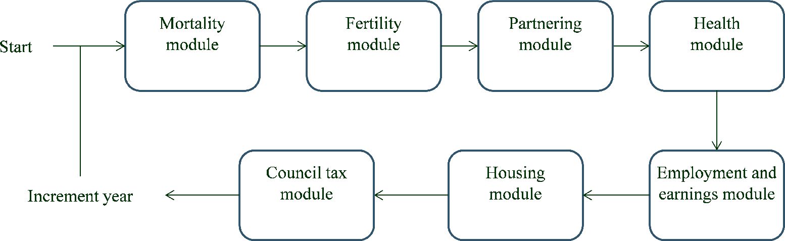

Microsimulation approach.
The microsimulation approach requires us to specify a set of parametric models for the nature of transitions over time. The specification of these models (and the order in which variables are modelled) need to be reasonable. In addition, the microsimulation approach does not avoid the problems of cohort differences that affect the splicing approach (although by scaling our transition probabilities as we discuss below, we can mitigate them) and so further assumptions are needed. In particular, if we are to estimate next period’s transition probabilities for characteristics Y on the basis of current information only, using data from cohorts other than the baby-boom cohort we require that
which is equivalent to the cohort independence assumption (5) made in the splicing approach
and the Markov assumption (6)
We do not however require the backward matching assumptions that we made for the splicing approach as we only model transitions going from younger to older ages. For more details, see (Kim et al., 2014).3 In the microsimulation approach, we have also found it relatively simple to relax the Markov assumption for some processes by including additional lags of variables when modelling transition probabilities (particularly for earnings and employment as we discuss below). Something similar could in principle be done to relax the Markov assumption in the splicing approach, though at the cost of making it harder to find matches (and by reducing the pool of potential donors, worsening the match quality for other variables we match on).
Estimation equations.
| Outcome | Method | Subsamples | Independent variables |
|---|---|---|---|
| Mortality | Logit | Cubic in age, dummy for receipt of disability benefits, couple status, education dummies and earnings quintile | |
| Child arrival | LPM | Run separately for women in couples and single women | For childless women: quadratic in age, dummy for ever had kids, number of kids ever had For women in couples: as for childless but also banded number of kids (0,1,2, and 3 or more) in household, age of youngest child, age of youngest child interacted with age |
| Child departure | LPM | Run separately by age of child (16–19) | Dummies for mothers and fathers education |
| Partnering | Logit | Run separately for 3 education groups and sex | Quartic in age, dummy for employed last period, dummies for number of kids in household (0,1,and 2 or more), dummies for couple status in previous three periods, dummy for single status last period interacted with age |
| Separating | Logit | Run separately for own education and sex | Quartic in age, employed last period, partner employed last period, dummies for banded number of kids in household (0,1,and 2 or more), cubic in current relationship length, age of youngest child, dummy for education same as partner |
| Health (IB and DLA receipt) | Logit | For IB: quartic in age, 4 lags of employment status (interacted), 4 lags of IB status (interacted) earnings quartile last period For DLA: quartic in age, 4 lags of employment status (interacted), 4 lags of DLA status (interacted) earnings quartile last period and 2 lags of IB status | |
| Renter (21 and over) | Logit | Run separately for current owners and current renters and for over and under 21s | Age of head of household, education of head of household, earnings quintile last period of head of household, banded number of kids (0,1,2 or 3 or more), couple status, relationship length dummy for rented last period, 4 lags of ownership status |
| Rank in rent distribution (21 and over) | OL | Run separately for owners, and renters in each of 5 rent quintiles | Age of head of household, education of head of household, earnings quintile last period of head of household, banded number of kids (0,1,2 or 3 or more), couple status, relationship length dummy for rented last period, 4 lags of ownership status |
| Renter status and rank (under 21) | MNL | Age of head of household, Age of head of household squared, | |
| Council tax band | OL | Run separately for each of 8 possible prior bands | cubic in age, banded number of children (0,1,2,3, 4 or more) renter status earnings quartile of household head, employment status |
-
Notes: LPM = Linear probability model, OL = Ordered Logit, MNL = multinomial logit.
Estimation equations for employment and earnings.
| Outcome | Method | Subsamples | Independent variables |
|---|---|---|---|
| Employment (22 and over) | Logit | Run separately for males and females, by employment in prior wave and by employment 2 waves ago | Education dummies, quartic in age, age-education interactions, dummy for over state pension age, dummy for having kids, dummy for couple status, dummy for having kids under 5, kids under 5 interacted with cubic in age, 3 lags of full-time status, banded number of kids (0,1,2 and 3 or more), couple status, couple-age interaction, lagged full-time status, lagged earnings rank,dummies for earnings quartiles (and 5 lags), employment status 3, 4,5 and 6 waves ago (and interactions), lagged disability status |
| Earnings quartile and part-time/full-time status (22 and over) | MNL | Run separately for each of 5 possible prior states: in part-time work, in full-time work and in 4 earnings quartiles and separately for males and females | Education dummies, quartic in age, age-education interactions, dummy for over state pension age, dummy for has kids, couple status, dummy for kids under 5, 3 lags of full-time status, current earnings rank (and 3 lags), 3 lags of earnings quartile dummies, 3 lags of employment status (interacted) |
| Employment and earnings (under 22) | MNL | Run separately for each of 6 prior possible states: unemployment, in part-time work, in full-time work and in 4 earnings quartiles | Sex, education dummies, dummy for has kids and age |
| Earnings rank within ‘bin’ (20 and over) | OLS | Run separately by prior state and sex | cubics in 4 lagged (within bin) ranks interacted with cubic in age, education dummies, dummies for ‘bin’ in previous 4 periods |
| Earnings rank within ‘bin’ (under 20) | OLS | Run separately by prior state and sex | cubics in lagged (within bin) ranks interacted with cubic in age, education dummies |
-
Notes: MNL = multinomial logit.
4.2 Scaling BHPS transition probabilities
In this section, we describe the scaling procedure we use to bring our profiles of our simulated individuals closer to the experiences of the baby-boom cohort.
Our aim is to replicate the experiences of the baby-boom cohort, in terms of employment rates, partnering and separation rates and so on. The problem is that we do not have panel data that covers all the years of that cohort. Instead, we have to make use of data from later cohorts when estimating transitions at younger ages in the BHPS and earlier cohorts when estimating transitions at older ages. Differences across cohorts may mean that these individuals do not provide a realistic representation of what happened to baby-boomers. For example individuals from later cohorts may be less likely to partner, may have fewer children and may have them later. However we do observe the evolution of these variables in a succession of cross-sections from the LCFS. This can be used to adjust estimates of transition probabilities based on the BHPS such that the transitions are consistent with the aggregate levels of the baby-boom cohort observed in the LCFS. This is something that is relatively easy to implement in the microsimulation approach, but is much harder to do in the splicing approach.
We start by noting that by the law of total probability gives us
where is the probability of being in state in i in period t (e.g being employed), and denotes the probability of moving from state i in period t to state j in period t +1. can be observed in the LCFS data, but the elements of the transition matrix (what we are interested in) are unknown. Since there are more unknowns than equations, the system does not have a unique solution. In order to choose from possible solutions, we choose the solution that is closest to the transition matrix estimated from the BHPS. We do this by minimising the norm of log differences between candidate transition matrices and transition matrices estimated from the BHPS. This gives us the smallest multiplicative factor that we would need to apply to our transition probabilities to reach the observed probabilities of being employed and so on in the LCFS data.4 The resulting transition probabilities are used to produce the correct proportions for couples, renters, and employment.5
So far, we have been describing the scaling procedure as if it is applied once at the aggregate level. We can, however, scale separately for different population cells. For instance, we can scale transition matrices to match employment rates separately for those with children and those without. This allows us to capture differences in the likelihood of parents being employed in our cohort of interest relative to the cohorts observed in the BHPS. Table 3 sets out the cells within which we match. Adopting this approach means that the scaling factors applied to each of the variables we are adjusting will vary by cell, and year.
Cells within which probabilities are matched to the LCFS.
| State | Cells |
|---|---|
| Couple | Age, year, sex, has children |
| Renter | Age, year |
| Employed | Age, year, sex, has children |
We scale the mortality rate using a simpler method. For this we take data from the Office for National Statistics Life Tables which provide average mortality rates for men and women at different ages for different birth years. We then use the difference between these and average mortality rates for individuals in the BHPS to scale mortality rates as predicted by a logit regression on income, disability benefit receipt, education and couple status.
4.3 Partnering
In the simulation, the aim in the partnering module is to partner individuals within the simulated sample (i.e. if one individual has a partner then his partner will also be in the sample). Thus all matches are assumed to take place within the same (nine year) birth cohort. This is in contrast to the splicing approach where partnering within the sample was not feasible. We allow for assortative matching in the choice of partners on the basis of education level, such that university-educated individuals are more likely to match with other university-educated individuals than those with GCSEs or less are. In order to implement this, we match potential partners based on an index that depends on education level and a random shock:
where ed2 is a dummy for having a secondary-level education and ed3 is a dummy for having a tertiary-level education. The values of the unknown parameters β and σ2 are chosen such that the distance between the simulated three-by-three matrix of education group against partner education group is as close to the empirical one as possible.
Which potential couples are realised, and which actual couples are dissolved, depends on partner arrival and departure probabilities estimated from our panel data.6 New couples and newly single individuals do not return to the partnering market until the following period. These probabilities are then scaled to match the marriage rates observed in repeated cross-sections of the baby-boom cohort we are interested in (see Section 4.3). Each couple requires a male and a female, and so a mismatch in the numbers of each can lead to too few matches being formed relative to what what our estimated probabilities would imply. To avoid this happening, probabilities of partnering are scaled again to achieve the expected number of matches. Matches can only occur between individuals who are both aged 16 or older.
All matches are assumed to take place within the same cohort, however we also wish to allow for the fact that males in couples in the 1945–54 cohort seen in the LCFS are on average just over 2 years older than females. (This is important because it has a knock-on effect on the ages at which children are born). To achieve this, our simulated males are born in the years 1945–52 while females are born between 1947–1954. This means in each period that the marriage market will be composed of females that are on average 2 years younger than their male counterparts.
4.4 Employment and earnings
A standard regression model of earnings can accurately capture changes in means and variances of earnings dynamics over time. However, as pointed out in (Bowlus & Robin, 2012), they suffer from the drawback of typically assuming that increases and decreases in earnings are equally likely regardless of where individuals are located in the earnings distribution. As a result, they will typically not capture key features of earnings mobility well (particularly mobility for the tails of the earnings distribution). Those in the top of the earnings distribution, for example, should be more likely to see their earnings fall than those at the bottom.
An alternative is to model transition probabilities between different segments of the distribution. We do this using a procedure that develops on that used in (Bowlus & Robin, 2012). Bowlus and Robin model transitions between segments of the residual distribution after a fixed-effects earnings regression. One concern with this approach is that when applied to a short panel, an earnings regression may conflate cohort and age effects on earnings levels (since those seen at older ages will tend to be from earlier cohorts). An alternative approach is to model movements within the earnings distribution of the cohort (i.e. earnings ranks). As with the splicing approach this would assume no cohort or period differences in the nature of transitions, but the exercise in Section 3.3 suggests that this assumption may not be too unreasonable (and in any case we would need to make a similar assumption if modelling residual transitions). Importantly, it would however allow for entirely arbitrary period and cohort effects in earnings levels.
To model movements in and out of the labour market, movements between part-time and full-time work, and movements around positions in the earnings distribution, we proceed through the following three steps:
Determine employment status: We estimate transition matrices for employment status separately for males and females and according to individuals’ employment status over the previous two waves. The probabilities making up this matrix are estimated through a set of logit models which include several lags of employment status (and interactions thereof) to help us match the high persistence of employment status observed in the data. They are also scaled so as to match the observed unemployment rates at different ages for the baby-boom cohort in the cross-sectional LCFS data (as discussed above).
Place the individual in an earnings ‘bin’: Once an individual’s employment status is determined, we then place the individual in one of 5 possible states or ‘bins’: in part-time work, or in full-time work and in one of four different earnings quartiles. Distinguishing between part- and full-time work is important for the receipt of tax credits. We assume that part-time work corresponds to 20 hours per week and full-time work to 40 hours. To determine which bin an individual should be placed in we estimate multinomial logits from each of the six possible prior states i (which include unemployment)
(14)The set of covariates included in x includes a cubic in age, education, a dummy for whether individuals have children or not, and a dummy for whether they have children under the age of 5, sex (as well as various interactions of all of these), their current earnings rank (entering linearly) as well as lags of full-time and employment status and lagged earnings quartiles.
Determine the individual’s precise earnings rank: The results from these models can be used to estimate the probability of moving between unemployment, part-time and full-time work and the different income quartiles. However, it does not place individuals precisely within these quartiles. One approach is to deal with this is to match simulated individuals to real-world individuals who made the same transitions as they did and use these individuals’ new ranks to determine the simulated individual’s new locations (the approach adopted by Bowlus and Robin). We found that in our case we were better able to match the persistence in earnings ranks by using a parametric approach. We predict ranks using the following regression
(15)where ri,t the within-bin rank of individual i in period t, and is a dummy which equals one if the individual was located in bin j in period t - τ. Φ-1(.) is the inverse of the CDF of the normal distribution. Linearly predicting Φ—1(ri,t) (and then feeding this prediction through Φ(.)) ensures that the predicted within bin rank always lies between 0 and 1. The polynomial of past ranks (up to a cubic) included in this regression is also interacted with a cubic in age in order to help us match the differing persistence of earnings over the life-cycle. In our simulations, we add a normally distributed noise term with the variance of residuals seen in the data to a linear prediction made using (5) to match the variance of ranks observed in the data.
Younger individuals (who do not have all the lags needed to be included in the regression models mentioned so far) have their status determined by a multinomial logit (across our five possible bins and unemployment) and a within bin regression involving only one lag. Once we have individuals’ ranks in the earnings distribution we can then fill actual values of earnings using cross-sectional data for the relevant cohort from the LCFS. As in the splicing approach, this means we will automatically capture changes in inequality, means and variances and other moments of the cohort of interest.
4.5 Rent
For rental payments and ownership status, we adopt a very similar procedure to that for earnings. We first use the estimates of a logit to determine whether an individual is an owner or a renter. For those who are renters, we then use the estimates of an ordered logit to predict their rent quintile; controlling for education of the household head (assumed to be the male in any couple), a cubic in age for the household head, couple status, relationship length, banded number of children and several lags of past renter status and past quintiles of the rent distribution. Placement within rental quintiles is random (the variance of the rental distribution is not as great as that of earnings meaning the exact placement within quintiles matters less). If the lagged variables differ between two members of a couple, they are taken from the household head. For younger individuals for whom we do not have a complete set of lags (those under 21), we run a simpler multinomial logit to determine transitions across all the possible states.
4.6 Private pensions
For private pensions we combine information from two datasets. The first consists of estimates of the discounted value of future private pension incomes for individuals in the BHPS survey from (Disney, Emmerson, & Tetlow, 2007). These estimates give the present value of future incomes for individuals if had they retired in 2001 or earlier, as well as projections for the future value of private pension wealth if individuals had continued in their present employment status until state retirement age. They are calculated using information from the special module of questions on private pensions included in the 2001 wave of the survey.7 The second is a set of predicted future private pension incomes for individuals seen in 2008 of the English Longitudinal Study of Ageing (ELSA). These include projected income streams conditional on individuals beginning to draw their private pensions in different years from 2008 onwards. The authors are indebted to Rowena Crawford, Soumaya Keynes and Gemma Tetlow for producing these projections and sharing them with us. Details of their methodology can be found in (Crawford, 2012) with an example of their use in (Banks, Emmerson, & Tetlow, 2014).
The approach we follow allows us to match real-world private pension income profiles to our simulated individuals on the basis of their labour market histories and other characteristics. We implement it in the following steps (once our simulations have finished)
We first estimate a probability that a simulated individual will ever receive a private pension using an individuals’ characteristics in 2001. We do this by estimating a logit model in the BHPS for that year. This regresses a dummy for positive projected private pension wealth in 2001 on sex and education dummies (and interactions of these), dummies for the number of the previous 5 years the individual was employed and dummies for the individuals’ decile of a 5 year moving average of previous earnings ranks.
We then predict the 2001 private pension ‘wealth’ (defined in here as the discounted value of future private pension incomes) for those simulated individuals who are to receive private pensions. This is done using the results of a regression of pension wealth in 2001 on a cubic in age, education dummies (and interactions of these) sex, years employed and a moving average of past earnings in the BHPS to which we add a normally distributed noise term.
We then calculate the simulated individuals’ ranks in this distribution within cells defined by age and year and use these to match them to a future stream of private pension income at the same rank from the ELSA data within cells defined by cohort, sex and couple status in 2008 (or earlier if they retire before this).
An individual’s retirement age is defined as the maximum of the final age at which they stopped working and 55. The ELSA data only predicts pension income for those who retire from 2008 onwards. For those who retire earlier than this, we deflate pension profiles associated with their retirement age using average earnings growth between 2008 and the year of their retirement. Earnings growth is what would determine private pension income for prior years from a defined benefit final salary scheme. The matching procedure works well, with on average 100 potential matches for each individual and an average distance between the ranks of donors and recipients of less than 1 percentage point.
5. Validation
5.1 Summary statistics for the splicing approach
Table 4 shows some summary statistics for the life-cycles we construct using the splicing approach. We fully or partially construct just over 1,900 life-cycles, on average completing 88% of the years between 16 and 83 (or death). However, only 514 (26%) complete fully from age 16 until an individual’s verifiable death. This is because matches for individuals cannot always be found in some circumstances (with particular difficulties at older ages when attrition from the BHPS sample for reasons other than death may be greater). At each join point there are an average of just over 35 potential matches, and on average our synthetic life-cycles are composed of 8.48 different individuals. The standard approach to dealing with data where there is non-random attrition or non-response is to weight observations according to their sampling probabilities as calculated from more representative data (such as population censuses or administrative sources). In a cross-sectional dataset these can be based on characteristics observed in a particular survey year (such as current income, race, sex etc.). To ensure that our spliced individuals provide representative results however, weights would need to be applied to each complete life-cycle. These weights would need to depend not only on the probabilities of having observed each individual in our initial sample, but also the probability of successive splicing producing a complete life-cycle. Unfortunately, there is no source from which we could obtain such weights.
Summary statistics (splicing approach).
| Number of synthetic life-cycles | 1,952 |
| Number of individuals used in splicing | 5,806 |
| Average number of splices per life-cycle | 8.48 |
| Average number of possible matches at joins | 35.4 |
| Proportion of years 16–83 (or death) covered | 88% |
| Completed until death | 514 |
5.2 Quality of matches in the splicing approach
One test of the quality of our matches in the splicing approach is to compare the autocorrelations of spliced variables at joint points (across two ages when a splice occurs) and at non-join points for variables which we do not insist on a perfect match for. When matches are not perfect, there is likely to be a slight discontinuity in outcomes at join points, which will give rise to a lower autocorrelation than that observed when no join is made. Tables 5–8 compare the two sets of autocorrelations for different five-year age groups. Despite matching across many different dimensions, autocorrelations at match points are not too dissimilar from autocorrelations observed in the data. Our matching procedure is less effective at capturing autocorrelations for the ranks of the rent distribution and for ranks of the earnings distribution and hours for over 65 year olds (due to the fact that fewer earners are available for matches in these years).
Autocorrelations in ranks for earnings.
| Age group | Autocorrelations when N match occurs | Autocorrelations when N no match occurs | ||
|---|---|---|---|---|
| 16–23 | 0.58 | 1,115 | 0.63 | 5,010 |
| 24–29 | 0.69 | 1,202 | 0.82 | 5,401 |
| 30–35 | 0.75 | 1,114 | 0.85 | 6,265 |
| 36–41 | 0.84 | 1,173 | 0.88 | 6,832 |
| 42–47 | 0.81 | 1,110 | 0.88 | 7,440 |
| 48–53 | 0.77 | 694 | 0.87 | 7,578 |
| 54–59 | 0.76 | 1,052 | 0.87 | 6,102 |
| 60–65 | 0.73 | 787 | 0.85 | 3,140 |
| 66–71 | 0.36 | 119 | 0.68 | 1,299 |
Autocorrelations in ranks for partner’s earnings.
| Age group | Autocorrelations when N match occurs | Autocorrelations when N no match occurs | ||
|---|---|---|---|---|
| 16–23 | 0.45 | 410 | 0.66 | 1,228 |
| 24–29 | 0.64 | 998 | 0.78 | 4,046 |
| 30–35 | 0.76 | 913 | 0.86 | 5,261 |
| 36–41 | 0.67 | 1,015 | 0.83 | 5,829 |
| 42–47 | 0.78 | 924 | 0.83 | 6,041 |
| 48–53 | 0.75 | 560 | 0.80 | 6,312 |
| 54–59 | 0.67 | 832 | 0.80 | 4,862 |
| 60–65 | 0.50 | 526 | 0.73 | 2,493 |
| 66–71 | 0.34 | 134 | 0.68 | 969 |
Autocorrelations in ranks for hours worked.
| Age group | Autocorrelations when N match occurs | Autocorrelations when N no match occurs | ||
|---|---|---|---|---|
| 16–23 | 0.39 | 1,310 | 0.47 | 6,115 |
| 24–29 | 0.37 | 1,321 | 0.65 | 5,752 |
| 30–35 | 0.61 | 1,188 | 0.74 | 6,618 |
| 36–41 | 0.65 | 1,224 | 0.75 | 7,183 |
| 42–47 | 0.61 | 1,152 | 0.74 | 7,752 |
| 48–53 | 0.60 | 730 | 0.72 | 7,924 |
| 54–59 | 0.68 | 1,085 | 0.76 | 6,363 |
| 60–65 | 0.58 | 811 | 0.76 | 3,351 |
| 66–71 | -0.02 | 151 | 0.63 | 1,418 |
Autocorrelations in ranks for rent.
| Age group | Autocorrelations when N match occurs | Autocorrelations when N no match occurs | ||
|---|---|---|---|---|
| 16–23 | 0.54 | 529 | 0.70 | 2,324 |
| 24–29 | 0.69 | 446 | 0.82 | 1,893 |
| 30–35 | 0.40 | 295 | 0.78 | 1,418 |
| 36–41 | 0.37 | 226 | 0.78 | 1,334 |
| 42–47 | 0.61 | 259 | 0.77 | 1,477 |
| 48–53 | 0.70 | 195 | 0.79 | 1,476 |
| 54–59 | 0.50 | 180 | 0.77 | 1,209 |
| 60–65 | 0.50 | 142 | 0.78 | 980 |
| 66–71 | 0.63 | 103 | 0.76 | 558 |
There is no analog in the microsimulation approach for the above statistics. There are no join points over which difficulties can arise and of course all simulated life-cycles cover the whole period from childhood until death.
The following two subsections discuss measures which can be used to compare the performance of the two methods directly.
5.3 Life-cycle profiles
Figures 2–7 show how age profiles for males and females from our simulated and spliced individuals compare to those observed for the baby-boom cohort in the LCFS for couple status, parenthood, single parenthood, number of children, renters and employment.
The figures show that the microsimultion approach performs well. Averages from our simulations need not automatically match those in the LCFS even with our scaling procedure. For instance, even if we accurately reproduced probabilities of being in a couple for those who have children and those who don’t, the proportion of couples would not match those in the LCFS if we did not also have the correct probabilities of being a parent at each age. Nonetheless, the match between the simulated individuals and cross-sectional averages in the data is excellent for all variables and both sexes. A difference in employment rates between the simulations and the data for younger ages is due to the fact that we impose that all those who have not completed full-time education are unemployed. A similar difference in the proportion of parents who are single in Figure 5 is due to the fact that, for years when cohorts are unobserved, we set the marriage rate for under 18s to be zero.
Our splicing procedure also does a good job of matching the experiences of the baby-boom cohort for couple status (Figure 3), parenthood (Figure 4) and number of children (Figure 6). For other variables, the profiles of our spliced individuals are however a little different those from the baby-boom cohort, reflecting cohort differences between the baby-boomers and individuals we observe in the BHPS. For instance, our spliced individuals are much more likely to be single parents at younger ages (Figure 5) reflecting the increase in lone parenthood over recent decades. Female employment rates also tend to be higher for our spliced individuals at younger ages and lower at older ages (Figure 2). Male employment rates are however captured quite well (except at younger ages when our spliced individuals are more likely to still be in education than the baby boomers). Figure 7 perhaps best illustrates some of the problems that can be created by cohort differences between individuals in the BHPS and the baby-boomers. It shows the proportion of individuals renting at different ages. It is apparent that individuals in the baby-boom cohort were far more likely to rent than our spliced individuals at younger ages. This likely reflects changes in the pattern of tenure in the UK, in particular the so-called “right-to-buy” reforms introduced in the 1980 Housing Act which gave those who had been renting social housing for at least 3 years the right to purchase their homes at a substantial discount. The effect of the policy was to dramatically reduce the number of social renters and increase home ownership from 59% in 1983 to 69% in 2003 (Chandler & Disney, 2014). This explains why those from later cohorts who comprise the donors to our spliced individuals at younger ages tend to be much more likely to own than the baby-boomers were at the same ages. The difficulty of capturing such cohort differences in the splicing approach tends in our view to favour microsimulation.
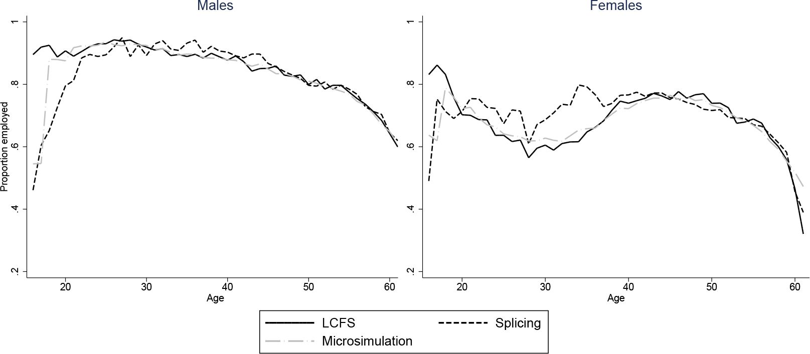

Employment: two approaches vs. LCFS, 1945–54 cohort.
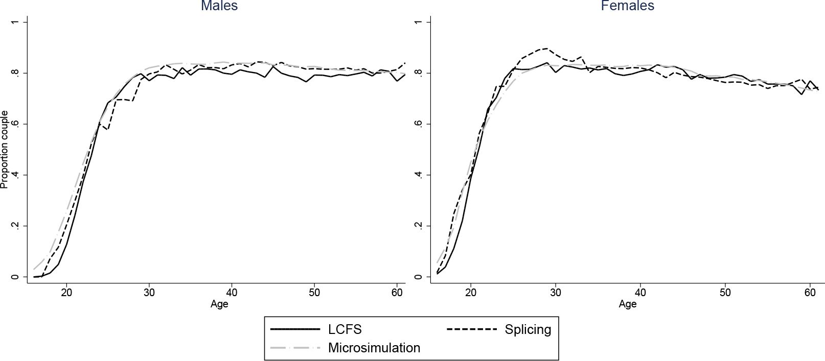
Proportion in couples: two approaches vs. LCFS, 1945–54 cohort.
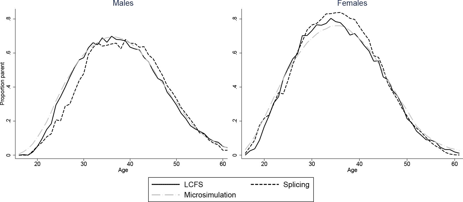

Proportion parents: two approaches vs. LCFS, 1945–54 cohort.

Proportion of parents that are single parents: two approaches vs. LCFS, 1945–54 cohort.
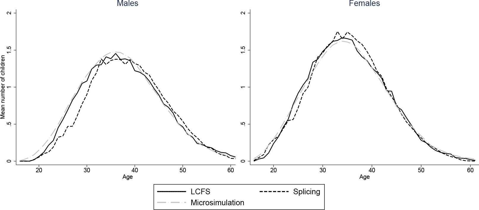

Number of children: two approaches vs. LCFS, 1945–54 cohort.
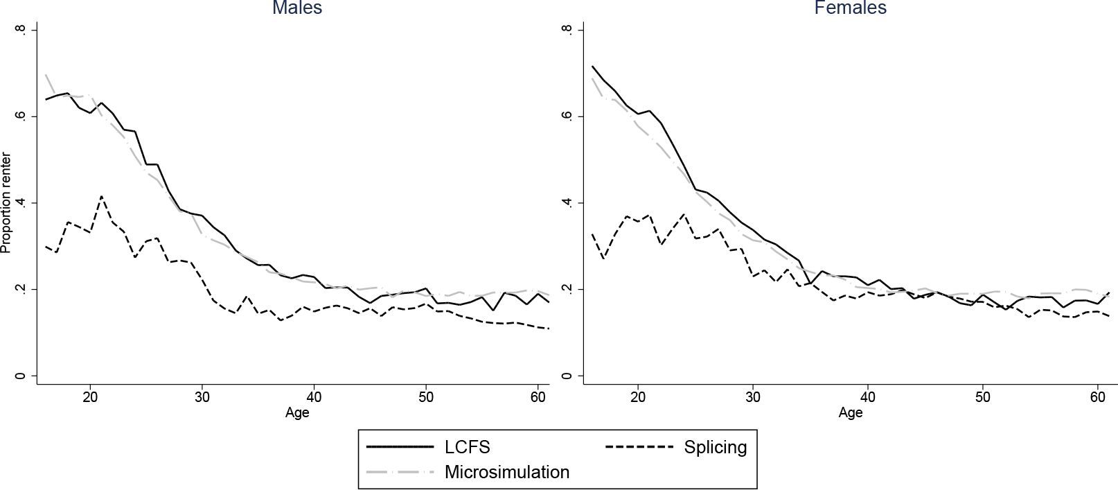

Proportion renters: two approaches vs. LCFS, 1945–54 cohort.
5.4 Transitions
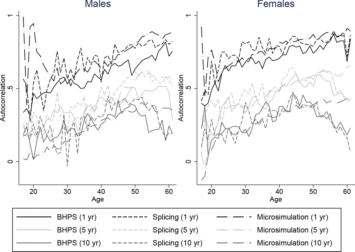
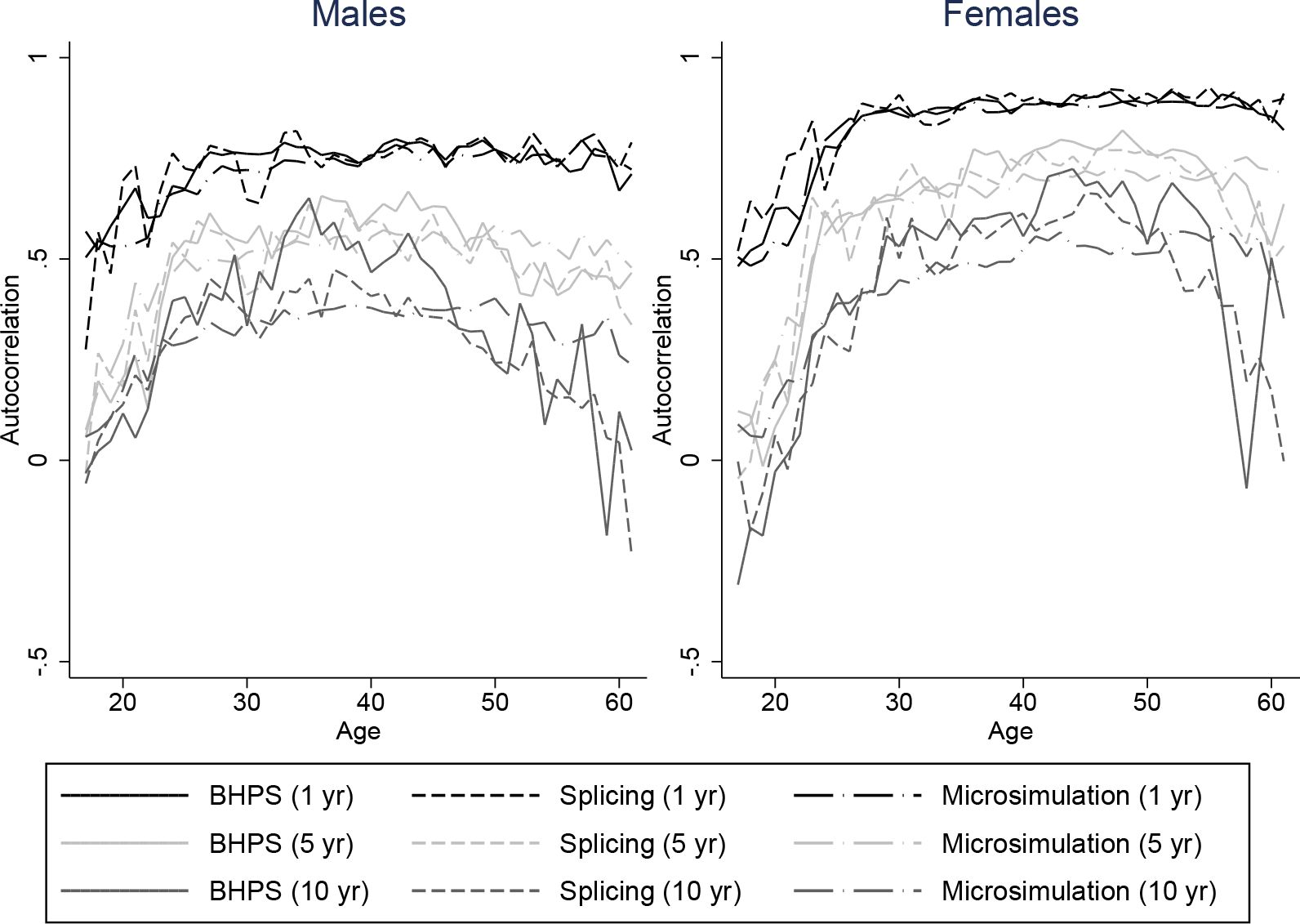
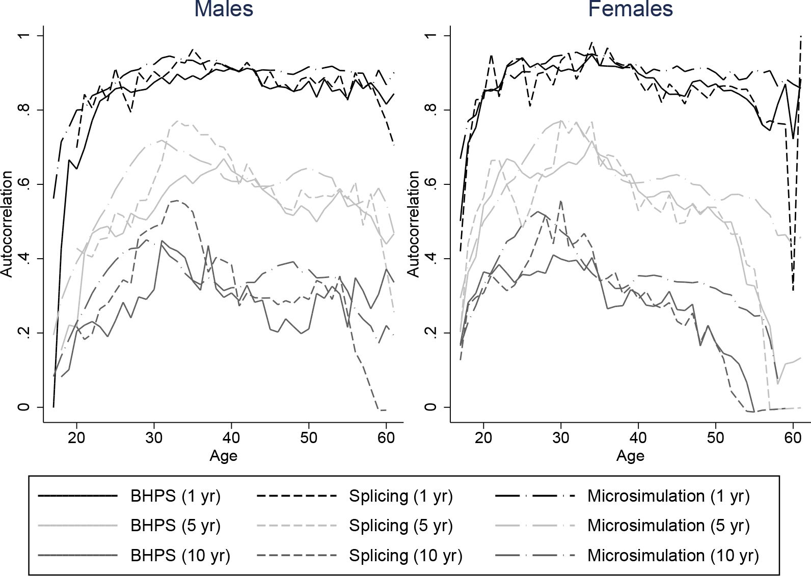
It is important that our spliced and simulated individuals do a good job at replicating the average lifetime profiles of the baby-boom cohort for our characteristics of interest. But since we intend to use our spliced individuals for distributional analysis of lifetime outcomes it is also important that the persistence of these variables match those of the data. Unfortunately we are not able to compare autocorrelations of our spliced and simulated individuals directly with individuals from the baby-boom cohort throughout the whole life-cycle, because we do not have access to a panel dataset covering the whole of the adult life-cycle for the baby boomers. Instead, we plot autocorrelations for our spliced individuals against those individuals seen in the BHPS. These are intended to show whether the transitions we obtain are plausible but cannot be used to see whether they are representative of the baby-boomers. Figures 8–11 plot autocorrelations for 1 year ahead, 5 years ahead and 10 years ahead for males and females from ages 16–65 for employment status, earnings ranks, couple status, and parent status.8
Our splicing procedure might not match the persistence of these variables in the BHPS if there are frequent joins or if matches only give appropriate continuations of earnings, couple status and so on for a few periods ahead. It is clear however that our spliced individuals match the transitions and persistence in the data well across all ages.
The processes experienced by our microsimulated individuals tend to have similiar persistence to those observed in the BHPS, although the difference is perhaps slightly greater than for the splicing approach. For example Figure 9 shows that for our simulated individuals, ranks in the earnings distribution are less persistent at middle ages for longer horizons than earnings ranks in the BHPS, and a little more persistent at older ages. The difference is a little larger for males than for females. Employment, couple, and parent status have similar persistence in our simulations to the data – even over 10 a year horizon. Overall the fit appears to be about as good as under the splicing approach.
Autocorrelations for employment status: two approaches vs. BHPS, ages 16–65.

Autocorrelations in earnings ranks: two approaches vs. BHPS, ages 16–65.

Autocorrelations for couple status: two approaches vs. BHPS, ages 16–65.

Autocorrelations for parent status: two approaches vs. BHPS, ages 16–65.
As an additional check on the performance of our simulations, we can compare our simulated and spliced individuals to those from the same cohort in the waves they are observed in the BHPS. Table 9 shows the proportions always employed, always unemployed, always in a couple and always single over 10 years from 1995 to 2004 (inclusive) in the BHPS, under the splicing approach, and in our simulations. The sample size in the splicing column differs from the number of synthetic life-cycles shown in Table 4 as some individuals die in the period 1995–2004 (and so are not observed over the whole 10 years).
Our microsimulations come very close to matching the proportions always employed and always in a couple although they appear to slightly underpredict the number of people always unemployed and always single. The splicing approach appears to a do a little better but the differences are not great.
Persistence of employment and couple status for 1945–54 cohort in BHPS, spliced life-cycles, and simulations (1995–2004).
| BHPS | Splicing | Microsimulation | |
|---|---|---|---|
| Always employed | 55.9% | 55.8% | 56.3% |
| Always unemployed | 12.4% | 10.2% | 11.4% |
| Always couple | 73.7% | 73.7% | 73.6% |
| Always single | 15.6% | 15.1% | 12.9% |
| N | 676 | 1807 | 4666 |
-
Notes: BHPS probabilities weighted for probability of attrition.
5.5 Validation summary
We judge our two approaches by their ability to replicate the experiences of the baby-boom cohort.
The splicing approach does well at recreating the transitions across the earnings distribution and between couple and tenure status that we observe in the BHPS, but is less good at replicating the average lifetime profiles of characteristics that differ greatly between cohorts. It is also not always feasible to find appropriate matches, meaning that only around a third of our spliced individuals produce complete life-cycles that run from age 16 until death. To the extent that the profiles which complete are non-random, this likely introduces a selection issue.
The microsimulation approach does not suffer from this particular drawback. Another key advantage over the splicing approach is that we are able to adjust transition probabilities estimated using panel data so as to match the age profiles we observe in a long-running cross-sectional survey. The match achieved in this respect is near perfect. Comparing the autocorrelations of variables over time suggests that our microsimulated processes also achieve a similar persistence to that observed in the BHPS.
Thus we favour microsimulation.
6. Summary
In this paper, we have outlined the practical steps we have taken to implement two different approaches to constructing full-adult life-cycles. Both approaches have strengths and weaknesses. The imputation literature provides helpful analogies when it comes to comparing the two methods. In this field, researchers often have a choice of imputing missing data using real-world data from similar individuals (a “hot-deck” imputation) or predicting it using a parametric approach estimated on the rest of the sample. The splicing approach has obvious similarities with the former method, while the microsimulation approach is closer to the latter. When is one approach to be preferred over the other? (Andridge & Little, 2010) compare these two approaches in a review of hot deck procedures, concluding from the available literature that “the relative performance of the methods depends on the validity of the parametric model and the sample size.” The hot deck approach is less vulnerable to model misspecification than the predicted outcome approach, but when the sample size is small, and the pool of potential matches diminishes, good matches can be difficult to find. Small sample sizes (or, for the same reasons, there being a large number of outcomes that need to be matched on) would therefore seem to favour the microsimulation approach. In a similar way, the splicing approach avoids the parametric assumptions of the microsimulation approach but matches may become less appropriate in smaller datasets where the pool of potential donors is smaller.
On balance we believe that for our application the microsimulation approach is to be preferred. While it is potentially sensitive to model misspecification, the assumptions it makes on transitions are slightly weaker than those of the splicing approach. In addition, it has the advantage that we can apply corrections to ensure that average outcomes are more similar to those experienced by the baby-boom cohort. Finally, the microsimulation approach is more amenable to simulating counterfactual outcomes (for instance, different future outcomes for the same individual).
Footnotes
1.
See (Andridge & Little, 2010) for a survey of hot-deck imputation.
2.
Earnings here includes self-employment income. We do not treat self-employment differently to other forms of employment, here or elsewhere.
3.
In the microsimulation approach, the Markov assumption needs to hold for all ages, while in the splicing approach it only needs to hold for ages from which we make forward matches (with the (7) required for ages when making backward matches).
4.
Probabilities are smoothed over time within cohort. Although this might limit the role of business cycles to contribute to changes in year to year employment for instance, it also prevents sampling variation spuriously adding volatility to our processes.
5.
It was not found necessary to scale child arrival rates.
6.
The lower of the two male and female probabilities are used to calculate the probability of separation for couples. This is to allow us to better match the persistence of couples observed in the data.
7.
The data itself was generously deposited in the UK Data Archive.
8.
The persistence of renter status is likely to be very different in the BHPS from the baby-boom cohort as a result of the much steeper declines experienced by the baby-boomers relative to those in later years illustrated in Figure 7. As a result we do not show the autocorrelations for this variable.
References
-
1
A review of hot deck imputation for survey non-responseInternational Statistical Review 78:40–64.
-
2
Effect of pensions and disability benefits on retirement in the uk. NBER Working Paper No. 19907.Effect of pensions and disability benefits on retirement in the uk. NBER Working Paper No. 19907., http://www.nber.org/papers/w19907.
-
3
Markov or not markov - this should be a question. Kiel Institute of World Economics Working Paper Series No 1086Markov or not markov - this should be a question. Kiel Institute of World Economics Working Paper Series No 1086.
-
4
Individual savings accounts for social insurance: rationale and alternative designsInternatinal Tax and Public Finance 15:67–86.
-
5
An international comparison of lifetime inequality: how continental europe resembles north americaJournal of the European Economic Association 10:1236–1262.
-
6
Housing market trends and recent policiesIn: C Emmerson, P Johnson, H Miller, editors. The IFS green budget. Institute for Fiscal Studies. pp. 90–125.
-
7
CBO’s long-term model: An overview. Congressional Budget Office Background paperCBO’s long-term model: An overview. Congressional Budget Office Background paper, http://www.cbo.gov/sites/default/files/06-26-cbolt.pdf.
-
8
ELSA pension wealth derived variables (waves 2 to 5): MethodologyUK Data Archive Study Number 5050 - English Longitudinal Study of Ageing.
-
9
What is a public sector pension worth?. IFS Working Papers W07/17Institute for Fiscal Studies.
- 10
-
11
Skatter och socialforsäkringer över livscykeln - en simuleringsmodell (Taxes and social insurance across the life cycle - a simulation model). Ds 1994, 86 (ESO)Stockholm: Swedish Ministry of Finance.
-
12
Assumptions needed to construct lifecycle dataAssumptions needed to construct lifecycle data, Unpublished Manuscript.
-
13
Inkomen en netto profijt van sociale zekerheid gedurende de levensloop uitkomsten van een trail (Transities van Inkomens tijdens de Levensloop) analyse (Income and net gains from social security during the life course)CPB Achtergronddocument 7.
Article and author information
Author details
Publication history
- Version of Record published: August 31, 2016 (version 1)
Copyright
© 2016, Levell & Shaw
This article is distributed under the terms of the Creative Commons Attribution License, which permits unrestricted use and redistribution provided that the original author and source are credited.